The Case for Specialization

When we think about the economics of production AI systems, there are three variables of interest: quality, cost, and speed. These variables are fundamentally bound together. For example, one can apply naïve scaling laws to increase the quality of a model’s prediction by doubling its parameter count and holding the training regime constant. However, this doubling of parameter count means the model’s forward passes will be slower. The speed of a forward pass can be increased with more compute, but at the cost of, well, cost.

With this paradigm in mind, consider the tremendous breakthroughs in the capabilities of coding agents over the past year. It is reasonable to assume a combination of improved training techniques as well as increased parameter count delivered this progress, evidenced by the dramatically rising costs of new models. But as frontier labs’ IPOs loom, Wall Street is beginning to ask about profitability and customers about costs. Amid this uncertainty, we present a post-training methodology that enables small, open-weight models to beat frontier intelligence at specialist tasks: in our case, extracting data from insurance loss runs (essentially cash flow statements on insurance policies). By taking a stringent approach to data curation and using simple off-policy training algorithms, we outperform frontier labs’ premier models on quality at twice the speed, all on a single B200 and at 1.5% of the cost of Fable’s completions on our test set. This isn’t a benchmark-only result: the model has been running in production for at least five enterprise customers since earlier this year.

• A perfect response means predicting every cell of our target table correctly; a longer document can produce several thousand cells.

More generally, we replicate frontier labs’ post-training methods at a smaller scale. Just as premier coding agents are trained by first curating vast but specialized coding datasets, we train a state-of-the-art insurance policy underwriting model by relying on iterations of labelling by human experts, sample rejection through deterministically verifiable invariants, and parameter-efficient finetuning methods. Our success also depends on having identified a sufficiently difficult problem for which data is hard to come by. There are many problems in the world beyond insurance underwriting that fit this mold. While most of the money behind AI is interested in making a 5T parameter model that both writes code and cures cancer, we remind ourselves that the story of economic history is a story that tends towards specialization, and we point to our loss runs model, which establishes an entirely new Pareto frontier across quality, cost, and speed, as evidence.

What makes this problem hard

A loss run is a table-heavy report of claims and policy history used for pricing future insurance policies (see here). These documents can be hundreds of pages long, and each insurer uses its own terminology and financial conventions. But underneath this surface variation, insurance accounting is a structured domain: field relationships follow known accounting identities, so a value missing from the document can often be inferred or calculated. There is exactly one correct canonical representation for a given loss run. Our task is to produce that representation as a JSON object, 4,000+ tokens on average. The rules that determine correctness are insurer-specific enough that writing them out in full would be tantamount to writing an entire textbook.

But even with this domain knowledge in hand, the data required to teach a model these rules is hard to get. Loss runs carry claimant names, medical details, and settlement amounts, so they are privacy-sensitive like other regulated financial and health records, and insurers treat their own loss experience as competitively sensitive on top of that, since it exposes underwriting performance to whoever sees it. These facts rule out the two usual workarounds for a data-hungry problem: open data (there is no public corpus to pretrain on), and synthetic data (since the data is private, there is no comprehensive baseline to synthesize from).

Long outputs, extensive rules, and data too sensitive to source at scale: this combination of factors lends itself to specialist post-training, and the methods we describe in this post would likely apply to any problem with this shape.

Results

Plotted against latency, our model sits in a distinct region from the frontier vendor curve rather than on an extension of it: a different regime on whichever of the three metrics you pick, at a fraction of the per-call cost of any frontier model we tested.

Percent perfect and the two accuracy metrics are computed at the document level (defined here). Percent perfect is the one that matters for production, since only a fully correct document can go straight through automation; macro and micro accuracy don’t tell you whether any single document is usable. A model at 80% average cell accuracy but 2% perfect documents is worse for production than one at 70% average accuracy but 50% perfect.

We also break results down by field, since a document-level number can hide which fields are dragging accuracy down. There’s no natural “perfect” at the field level (each field is right or wrong per row, no partial credit), so we report micro accuracy by field instead: our model against Fable 5, Gemini 3.1 Pro, and GPT-5.6-Sol, in the Field Analysis tab above. This is diagnostic detail, not the headline.

Our post-trained model leads on every field we measure, and the gap tracks how much insurer-specific knowledge a field demands, not how hard it is to read a table in general:

• Domain-specific fields show the largest gaps. Claim status (89.3% vs. 65.7–69.1% for Fable 5, Gemini 3.6 Flash, and GPT-5), claim type (82.0% vs. 59.3–67.1%), and line of business (92.9% vs. 85.5–88.8%) all depend on carrier-specific vocabulary rather than generic extraction.
• Financial fields show the same pattern at a smaller scale. Allocated expenses, total paid, total reserve, indemnity, and medical amounts run 4 to 15 points ahead, with total paid and total reserve the widest.
• Carrier identification fails on consistency, not just correctness. Across 130 carriers appearing at least three times in the eval set, our model uses one consistent string 86.2% of the time (1.16 variants/carrier); Fable 5, Gemini 3.6 Flash, and GPT-5 land at 61.5–73.1% (1.26–1.44 variants/carrier). Worst case, Gemini 3.6 Flash gave five different answers for Erie Insurance Exchange across its 129 occurrences: four name variants plus 15 outright misses.
• Carrier identification also fails on comprehension. One loss run lists Berkley Mid-Atlantic Group’s six underlying pool members by name. Sonnet 5, Haiku 4.5, and Gemini 3.6 Flash all reported that member list as the carrier instead of the pool name; our model correctly reported Berkley Mid-Atlantic Group. That a list of six carriers describes one pooled placement, not a prompt to enumerate, isn’t something a model can infer from the page text alone.

How much of this is post-training?

We also evaluated Qwen3.5-27B itself, before any post-training, on the same hardware and inference settings as our post-trained model. Its macro and micro accuracy, 80.6% and 79.9%, land in the same range as the frontier models we tested. Its percent perfect is 16.7%, the lowest of any model in this eval. The base model looks frontier-competitive on macro and micro accuracy, and falls to the bottom on the metric that actually predicts straight-through automation. Post-training accounts for the gap between 16.7% and 52.9%, larger than the gap to any frontier model we measured.

It’s also comparable on cost and latency: 18.0 seconds and $0.0062 per document for the base model, against 21 seconds and $0.0072 for ours, both from the same $0.16633/minute B200 rate amortized across our 8 parallel workers. If anything the base model is marginally faster and cheaper. Post-training’s advantage here is accuracy, not efficiency: we have no evidence it changed how efficiently the model answers, only what answer it gives. Thanks to Baseten for great GPU pricing and autoscaling, which allow us to win on cost in addition to quality.

How we actually curate the data

To achieve these results, we employ a variant of rejection fine-tuning (RFT) on LoRA adapters on a single H100. Our model generates initial completions from raw loss run documents, which we then pass through deterministic validators that check domain invariants, like total_incurred = total_paid + total_reserve - |recovery| or incident_date <= reported_date <= closed_date. Samples that pass are immediately used in iterated SFT training. Samples that fail are sent to human experts for correction rather than discarded, so we get expert signal on exactly the cases the model struggled with, instead of throwing them away. We like this approach for its simplicity: no policy gradients, no reward models, no advantage estimation. The relatively small size of our model and dataset enable us to retrain every few weeks, and as the model has improved, a growing fraction of samples pass validation without human correction, meaning the training signal is increasingly dominated by unmodified on-policy outputs.

Where we diverge from standard RFT is the reject path. Most published RFT/RAFT/ReST pipelines simply discard candidates that fail verification; a recent critique of that approach (Step Rejection Fine-Tuning) notes that traditional RFT throws away unresolved trajectories even though they concentrate exactly the cases a model struggles with. We don’t discard them. A rejected candidate goes to a human, who fixes whichever of the annotation or the DSL rule was actually at fault, and the corrected example re-enters the training pool. That’s closer to DAgger’s correction loop from imitation learning, where a policy’s failures get queried out to an expert and the correction is aggregated back into training, than to plain rejection sampling. STaR makes a similar move for math reasoning: instead of discarding wrong answers, it re-prompts the model with a hint containing the correct one and trains on the resulting rationalization. Ours shares that instinct, don’t throw away exactly the examples where the model is weakest, but the repair comes from a human fixing the underlying rule or annotation, not the model correcting itself from a hint.

This is close in spirit to Baseten’s recent post-training work with Harvey on legal agents, which uses an iterative SFT stage on rubric-passing rollouts to bring a 27B open-weight model into the closed-source frontier band on Harvey’s Legal Agent Benchmark, followed by a GRPO reinforcement learning stage. Our pipeline stops at the iterative SFT stage and substitutes a symbolic domain-logic verifier for their rubric judge; we have not yet added an RL stage on top.

This is a useful data point for the industry: everybody wants to learn on-policy, for reasons from GRPO sample efficiency to avoiding forgetting (our post-train retains the base model’s tool use and reasoning). We bootstrap our model’s capability to bring the dataset more on-policy by means of a simple RFT-style loop that doesn’t require a reward model or policy gradients, with the benefit of dense token-level supervision. This has enabled us to move the insurance domain in-distribution in a manner that will enable our future RL-based rollout efforts to be more effective, since the post-trained model now produces a higher share of valid rollouts than previously.

Conclusion

Throughout this year, which saw huge improvements in frontier models, we have maintained our lead on loss run extraction, while frontier models stagnate on our benchmark across generations (GPT-5.6-Sol performs worse than GPT-5). But the point of our benchmark is not that, with adequate reasoning and agentic capabilities, Fable 5 or similar models could not be trained to extract data from loss runs better while maintaining its coding abilities. The point is that a truly “generally intelligent” model would just curate the data to post-train our model, and thereby solve this use case using minimal energy.

We currently serve this model on Baseten infrastructure, and are live in production across several customers. We’ve changed the way insurance underwriting operates, and hope others consider our methodology (and the low cost of compute through Baseten) to tackle other industry automation problems.

Appendix

Example Loss Run

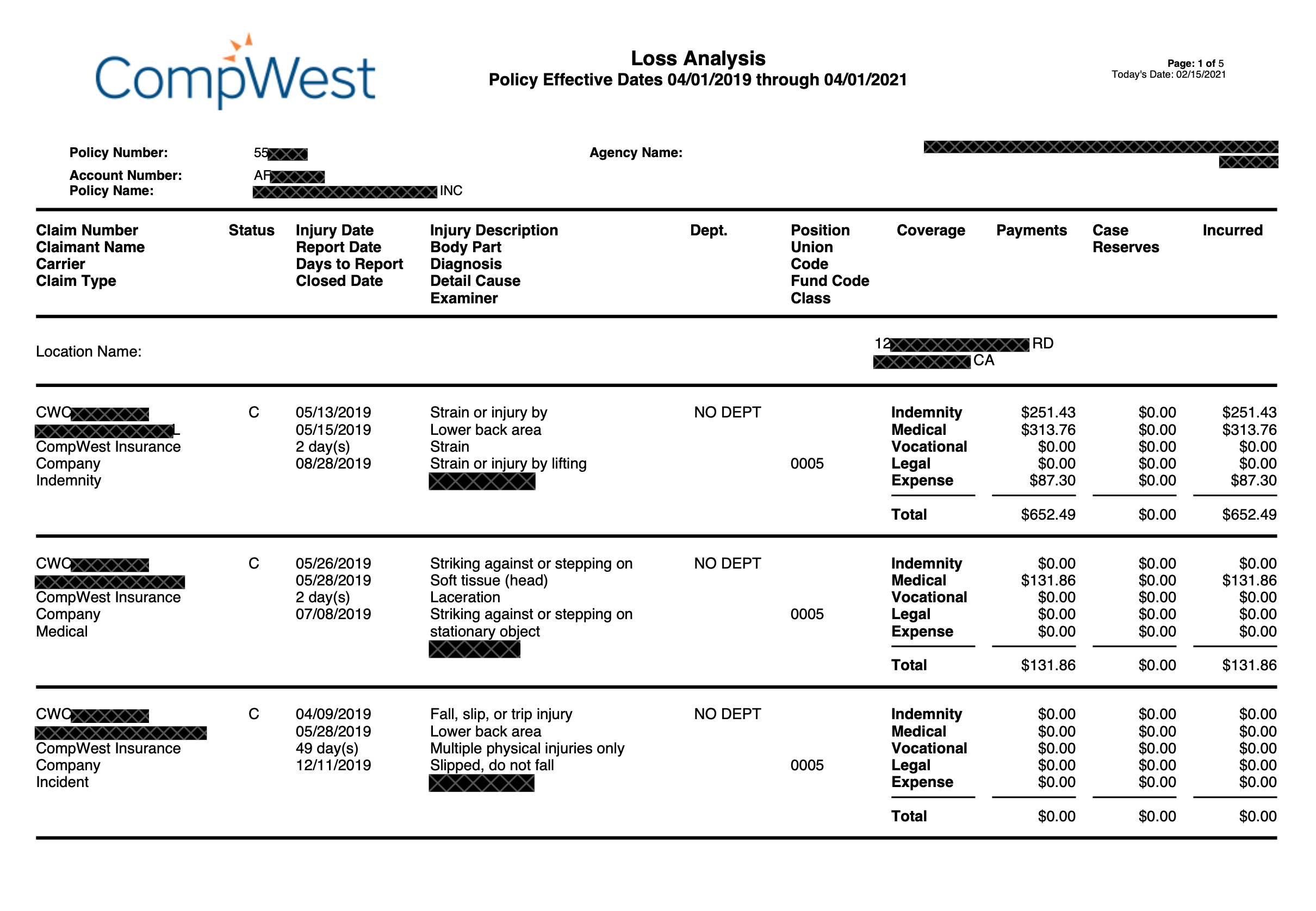
Each column stacks several fields into one cell rather than holding a single value. The dates column stacks Injury Date, Report Date, Days to Report, and Closed Date in that order, so 05/13/2019 is the injury date only because it’s first in the stack, not because of anything in the cell itself. The same holds for the claim-identity and financial columns: reading any single field correctly means counting its position and matching it back to the stacked header, not reading left to right.

Metrics

• Percent perfect. The share of documents extracted with zero cell errors, no partial credit. This is the number that determines whether a document can go straight through automation or has to be routed to a human, since there is no such thing as a “90% correct” filing:

$$ \text{PercentPerfect} = \frac{1}{N} \sum_{i=1}^{N} \mathbb{1}\left[\sum_{j=1}^{n_i} \text{Acc}(cell_{i,j}) = n_i\right] $$

• Macro accuracy. Cell-wise accuracy averaged per document, then averaged across documents, so every document counts equally regardless of size:

$$ \text{Macro} = \frac{1}{N} \sum_{i=1}^{N} \frac{1}{n_i} \sum_{j=1}^{n_i} \text{Acc}(cell_{i,j}) $$

• Micro accuracy. Cell-wise accuracy pooled across the entire evaluation set, so larger documents contribute proportionally more cells:

$$ \text{Micro} = \frac{\sum_{i=1}^{N} \sum_{j=1}^{n_i} \text{Acc}(cell_{i,j})}{\sum_{i=1}^{N} n_i} $$

where $N$ is the number of documents and $n_i$ is the number of cells in document $i$’s extraction.

Every metric below carries a 95% confidence interval, from resampling the 346-document eval set with replacement 10,000 times. That bounds sampling noise on this fixed set, not variance from retraining with a different seed, which we haven’t measured.

Reproducibility

• Base model: Qwen3.5-27B
• Training method: iterative rejection sampling fine-tuning (RFT/RAFT/STaR lineage) on the accept path; a DAgger-style human-correction loop on the reject path, where rejected candidates are corrected and re-enter the pool rather than being discarded; gated by an insurer-specific domain-logic validator (structural + business-rule DSL); no reinforcement learning stage
• Training hardware: single H100, ~1 week, sequences up to 32K tokens
• Inference hardware: single B200, 8 parallel workers, 32K context, BF16 with FP8 KV cache, speculative decoding up to 10 tokens ahead via multi-token prediction
• Evaluation set: 346 held-out loss run documents, 12 lines of business, 2 table schemas (Claims and Policy Loss Runs)
• Metrics: percent perfect (headline); macro and micro accuracy (diagnostic), defined above
• Confidence intervals: 95% bootstrap CIs, document-level resampling with replacement, 10,000 resamples per model per metric; covers sampling variance over the fixed 346-document set only
• Baselines: Claude Fable 5, Opus 5, Opus 4.8, Sonnet 5, Sonnet 4.6, Haiku 4.5; GPT-5, GPT-5.6-Sol, GPT-4.1; Gemini 3.6 Flash, Gemini 3.5 Flash, Gemini 3.1 Pro, Gemini 3.1 Flash Lite; Qwen3.5-27B (base). Pricing confirmed as of August 2026.
• Reasoning effort: every baseline that supports a thinking/reasoning mode is reported at medium effort, including Gemini 3.1 Pro and Gemini 3.1 Flash Lite, which we previously reported non-thinking; standardized here so every frontier baseline uses the same convention
• Cost methodology: base and post-trained Qwen3.5-27B are both served on B200 hardware, on matched inference settings, at $0.16633/minute; cost per document is per-document serving time at that rate, divided across our 8 parallel workers, not a metered API price like the other baselines