LLM Calibration and Confidence Estimation

This review wouldn’t be possible without the following review papers:

• A Survey of Confidence Estimation and Calibration in Large Language Models

Basic Concepts

Confidence and uncertainty are two sides of the same coin:

• Confidence refers to the degree of belief that a prediction or statement is correct.
• Uncertainty quantifies the degree of doubt about the correctness of a prediction or statement.

High confidence implies low uncertainty, and vice versa. In fact, the two are complementary in that they sum to 1.

Types of Confidence

Confidence can be categorized as relative or absolute:

• Relative Confidence: This refers to a model’s ability to rank samples by their likelihood of being correct. A model exhibits relative confidence when it can produce a scoring function, $\text{conf}(\mathbf{x}_i, \hat{y}_i)$, such that:

  $$ \text{conf}(\mathbf{x}_i, \hat{y}_i) \leq \text{conf}(\mathbf{x}_j, \hat{y}_j) \iff \text{P}(\hat{y}_i = y_i | \mathbf{x}_i) \leq \text{P}(\hat{y}_j = y_j | \mathbf{x}_j) $$

  Here, $\hat{y}_i$ is the model’s prediction for sample $\mathbf{x}_i$, and $y_i$ is the true label for $\mathbf{x}_i$.

• Absolute Confidence: This refers to the model’s ability to produce a well-calibrated confidence score. The model achieves absolute confidence when the scoring function, $\text{conf}(\mathbf{x}_i, \hat{y}_i)$, satisfies:

  $$ \text{P}(\hat{y}_i = y_i | \mathbf{x}_i) = \text{conf}(\mathbf{x}_i, \hat{y}_i) $$

  This implies that for all predictions where the model’s confidence score is $q$, the proportion of correct predictions should also be $q$:

  $$ \text{P}(\hat{y}_i = y_i ,|, \text{conf}(\mathbf{x}_i, \hat{y}_i) = q) = q $$

Calibration

When discussing calibration, we generally refer to absolute calibration. A model is well-calibrated if its predicted probabilities match the true probabilities.

Quantifying Calibration

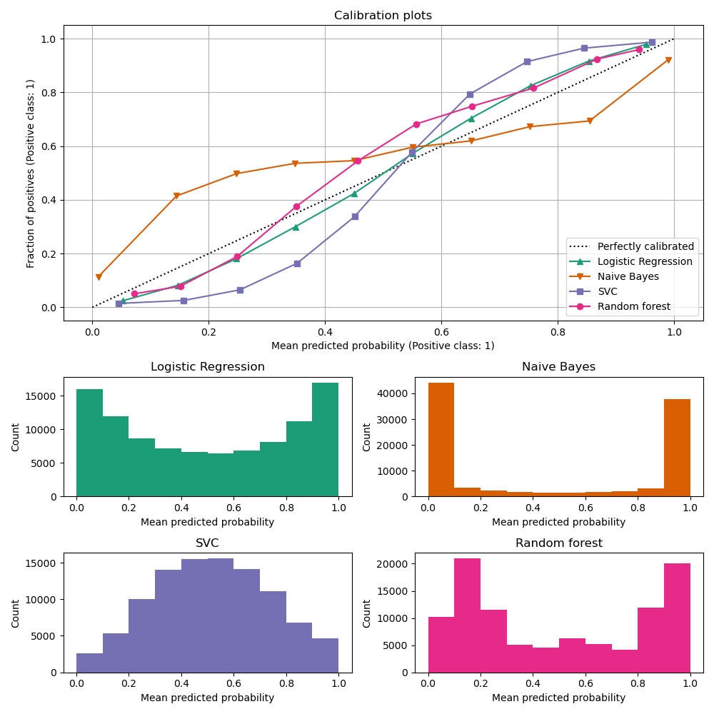
Reliability Diagram / Calibration Curve

A reliability diagram is a visual representation of a model’s calibration. It plots the average confidence of a model against the accuracy of the model. Specifically, the x-axis represents the predicted confidence scores (usually grouped into bins), and the y-axis represents the empirical accuracy for those bins.

The reliability diagram is a useful tool for understanding how well a model’s confidence scores align with the true probabilities. However, one should always pair a reliability diagram with the distribution of confidence scores so as to avoid drawing incorrect conclusions. This is because a lack of calibration within a bin can be aggravated by the lack of samples in that bin.

Frequently, the reliability diagram includes a diagonal line that represents a perfectly calibrated model. A model is well-calibrated if its reliability curve is close to this diagonal line.

See Calibration curves with an example in scikit-learn.

Expected Calibration Error (ECE)

Due to the continuous nature of confidence scores, we can never achieve perfect calibration. However, by discretizing the confidence scores into $M$ bins, we can approximately measure the calibration of a model. The Expected Calibration Error (ECE) is defined as:

$$ \text{ECE} = \sum_{m=1}^{M} \frac{|B_m|}{N} \left| \text{acc}(B_m) - \text{conf}(B_m) \right| $$

Here, $B_m$ is the set of samples whose confidence scores fall into the $m$-th bin, $N$ is the total number of samples, $\text{acc}(B_m)$ is the accuracy of the model on $B_m$, and $\text{conf}(B_m)$ is the average confidence of the model on $B_m$.

From this definition, we can see that the ECE is a weighted average of the differences between the accuracy and confidence of the model in each bin. The differences are computed using the absolute value (L1 norm). It is a representation of the average case behavior of the model.

Maximum Calibration Error (MCE)

The Maximum Calibration Error (MCE) is defined as:

$$ \text{MCE} = \max_{m} \left| \text{acc}(B_m) - \text{conf}(B_m) \right| $$

The MCE is the maximum difference between the accuracy and confidence of the model in any bin. It is a representation of the worst case behavior of the model. As such, it is a much more sensitive metric than the ECE, as a single poorly calibrated bin can lead to a high MCE.

Issues with ECE and MCE

While the ECE and MCE are useful metrics for quantifying calibration, they have some limitations:

• They are sensitive to binning; the width of the bins can affect the calculated values, and so do the number of bins.
• They fail to fully capture the variance of samples within each bin.

Because of this, some have worked to develop more robust variants of these metrics. A good example of this is Nixon et al.’s 2019 paper. This introduces:

• Static Calibration Error (SCE): A multiclass generalization of the ECE.
• Adaptive Calibration Error (ACE): A version of ECE that focuses on an adaptive range of bins. Instead of uniformly dividing the range of confidence scores into equal-width bins, ACE uses a dynamic binning strategy that seeks to construct bins with a similar number of samples.
• Thresholded Adaptive Calibration Error (TACE): A variant of ACE that introduces a threshold to filter out bins with few samples. Only predictions above a certain threshold are considered for calibration.

Other valuable metrics include using the area under the receiver operating characteristic curve (AUC-ROC) and the area under the accuracy-rejection curve, both of which can be helpful in assessing a confidence score’s ability to differentiate between correct and incorrect predictions. Ocassionally, the Brier score is also used to measure calibration, or the negative log-likelihood of the model’s predictions.

Further Reading on Calibration Basics for Neural Networks

• Predicting good probabilities with supervised learning
• On Calibration of Modern Neural Networks
• Measuring Calibration in Deep Learning

Confidence Estimation Methods

Here, we highlight various methods for producing a function $\text{conf}(\mathbf{x}_i, \hat{y}_i)$. This is irrespective of the underlying model’s calibration, and solely focuses on just the confidence estimation component.

Logit-based Confidence

Logit-based confidence estimation is the practice of using the logits produced by a model as a proxy for how confident the model is in its predictions. While it may be more obvious for classification models, it is less so for large language models (LLMs) that may output a multi-token sequence. At this point, one must ask whether to use the logits of the final token, the sum of the logits, or some other aggregation of the logits.

Additionally, this type of confidence estimation further encapsulates all methods that derive their certainty from some measure of the model’s output, such as the entropy of the model’s predictions or the gap between the highest and second-highest logits.

• Pros:
  • Simple to implement.
  • Can be used with any model that produces logits.
• Cons:
  • Logits may not directly translate to well-calibrated probabilities, especially in models not trained with calibration in mind.
  • Can be sensitive to the model’s architecture and training data.
  • Has not been shown to be effective, especially for situations where the model’s output is a sequence of tokens.

Further Reading on Logit-based Confidence

• Look Before You Leap: An Exploratory Study of Uncertainty Measurement for Large Language Models
• Calibration-Tuning: Teaching Large Language Models to Know What They Don’t Know
• Teaching Models to Express Their Uncertainty in Words

Ensemble-based Confidence

Ensemble methods estimate confidence by training multiple models and aggregating their predictions. The intuition is that if multiple models agree on a prediction, then the prediction is likely to be correct. Disagreements between models indicate uncertainty.

Deep Ensembles

Deep ensembles are a type of ensemble method that train multiple neural networks on the same dataset. Each network is initialized with different random weights and trained independently. The final prediction is made by averaging the predictions of all the networks.

The idea is that by having randomness from the initialization and the training process, the ensemble can capture different aspects of the data distribution. This can help to improve the model’s generalization and provide better confidence estimates.

• Pros:
  • Can provide well-calibrated confidence estimates.
  • Can improve the model’s generalization.
  • Is well-grounded in theory.
• Cons:
  • Requires training multiple models.
  • Can be computationally expensive to train and deploy.
  • Impractical for large models or datasets.

Further Reading on Deep Ensembles

General background on deep ensembles can be found in the following papers:

• Simple and Scalable Predictive Uncertainty Estimation using Deep Ensembles
• Uncertainty Quantification and Deep Ensembles
• Deep Ensembles Work, But Are They Necessary?

Some interesting (but not accepted in peer-reviewed conferences) works where the idea of deep ensembles and LLMs/LoRA is discussed:

• LoRA ensembles for large language model fine-tuning
  • Rejected from ICLR 2024
• Uncertainty quantification in fine-tuned LLMs using LoRA ensembles
• LoRA-Ensemble: Efficient Uncertainty Modelling for Self-attention Networks

Monte Carlo Dropout

Monte Carlo Dropout is a technique that uses dropout at test time to estimate model uncertainty. Dropout is a regularization technique that randomly sets some neurons to zero during training. Typically, at test time, dropout is turned off, and the model makes predictions using the full network. However, with Monte Carlo Dropout, dropout is left on at test time, and multiple predictions are made by sampling from the dropout mask. The final prediction is made by averaging the predictions.

MC Dropout can be seen as a type of deep ensemble, where the ensemble members are different subnetworks of the same model. It is theoretically equivalent to approximating the Bayesian posterior of a neural networkc (see Gal and Ghahramani @ ICML 2016). Where MC Dropout lacks the need to train multiple models, it suffers from a need to make multiple inferences per each data point. This drives up the computational cost of using MC Dropout for confidence estimation.

• Pros:
  • Can provide well-calibrated confidence estimates.
  • Can be used with any model that uses dropout.
  • Is well-grounded in theory.
• Cons:
  • Requires making multiple inferences per data point.
  • Can be computationally expensive to use.
  • May be prohibitively slow for large models.

Further Reading on Monte Carlo Dropout

• Dropout as a Bayesian Approximation: Representing Model Uncertainty in Deep Learning
• LoRA Dropout as a Sparsity Regularizer for Overfitting Control

Density Estimation

Usually density-based methods require making some set of assumptions about the model and its training data. A simple assumption is that the model will be more confident in regions of input space where the model has seen training data.

A common idea is to place Gaussian distiributions around training data points and to use a test-time data point’s distance from the training points as a surrogate for confidence. Usually this distance is exponentiated. This is highly dependent on the kernel used to measure distance, and the representation of the data points. Furthermore, in high-dimensional spaces, distance metrics can become less meaningful due to the curse of dimensionality, making density estimation less reliable.

• Pros:
  • Can provide well-calibrated confidence estimates.
  • Can be used with any model.
• Cons:
  • Requires making assumptions about the data distribution.
  • Can be sensitive to the choice of kernel and hyperparameters.
  • May not be well-suited for high-dimensional data.
  • Not suitable for large datasets, as typically requires storing all training data.

Confidence Learning

This involves training a model to predict its own confidence. An example of this is shown in a 2018 paper by DeVries and Taylor. Specifically, this involves adapting how a model is trained to include an additional output branch that predicts the model’s confidence. The model’s final prediction is a combination of its initial prediction and the confidence estimate, effectively adjusting its output based on how confident it is. Additionally, the confidence is log-penalized to prevent the model from predicting zero confidence (which would achieve perfect performance per the loss function).

• Pros:
  • Can provide well-calibrated confidence estimates.
  • Seems promising for out-of-distribution detection.
• Cons:
  • Requires modifying the model’s architecture and training procedure.
  • May be sensitive to hyperparameters.
  • May not be well-suited for all models.
  • Hasn’t been widely applied to LLMs.

Verbal Ellicitation of Confidence

When dealing with LLMs, it may be useful to ask the model to generate a confidence score. This can be done by asking the model to generate a confidence score for a given input or asking it otherwise specify, verbally, how confident it is in its prediction. Sometimes options are given in the prompt to guide the model towards stating its confidence a certain way.

• Pros:
  • Can provide a direct measure of the model’s confidence.
  • Can be used with any LLM.
• Cons:
  • May not be well-calibrated.
  • May require human intervention.
  • May not be suitable for all tasks.
  • Lacks a theoretical grounding, and may yield inconsistent results.
  • The elicited confidence may be influenced by the prompt and may not reflect true uncertainty.

Further Reading on Verbal Elicitation of Confidence

• Teaching Models to Express Their Uncertainty in Words
• Reducing Conversational Agents’ Overconfidence Through Linguistic Calibration
• Just Ask for Calibration: Strategies for Eliciting Calibrated Confidence Scores from Language Models Fine-Tuned with Human Feedback

Calibration Methods

Now that we’ve talked through various methods for estimating confidence, we can discuss methods for calibrating a model to produce well-calibrated confidence scores.

In-Training Calibration

Loss Functions

One way to improve a model’s calibration is to use a loss function that encourages the model to produce well-calibrated confidence scores. This is, typically, of limited-use for LLMs, as in-training calibration tricks frequently relies on adapting a model’s full training procedure in ways not typically considered for LLMs.

Focal Loss

Focal loss is a loss function that upweights the loss for samples that are hard to classify, and downweights the loss for samples that are easy to classify. This can help to improve the model’s calibration by focusing on the samples that the model is less confident about. It was originally proposed to address class imbalance in object detection tasks.

Correctness Ranking Loss

A loss function that incorporates ranking will include a term that looks at a batch of predictions and penalize a model for insufficiently ranking and separating correct and incorrect predictions.

• Confidence-Aware Learning for Deep Neural Networks

Entropy Regularization Loss

This is a penalization term that encourages a model to avoid being too confident. Entropy regularization adds a term to the loss function that penalizes overconfident predictions by encouraging higher entropy (more uncertainty) in the output distribution. This loss encourages the model to assign higher confidence scores to correct predictions than to incorrect ones, effectively learning to rank predictions based on correctness.

• Regularizing Neural Networks by Penalizing Confident Output Distributions

Label Smoothing

Label smoothing is a regularization technique that replaces the hard targets with a smoothed distribution. This can help to improve the model’s calibration by reducing the model’s confidence in its predictions.

• Rethinking the Inception Architecture for Computer Vision

This might be a simple way to improve calibration in LLMs, but we need to be cautious with how we go about it. Where we’ve seen this technique help with calibration, particularly with things such as machine translation, I have seen less evidence of its effectiveness in an instruction tuning approach. Before we leap to label smoothing, we should consider simple experiments to see if we maintain a similar degree of performance as well as improved calibration metrics if we apply label smoothing.

Data Augmentation

Data augmentation refers to any techqnique that artificially increases the size of the training data by applying transformations to the data. This can help to regularize the model and improve its calibration by exposing the model to a wider range of data.

Most frequently, we see data augmentation used in computer vision tasks. However, some people have developed ways to exploit techniques like MIXUP to improve calibration in LLMs.

• On the Calibration of Pre-trained Language Models using Mixup Guided by Area Under the Margin and Saliency
• EDA: Easy Data Augmentation Techniques for Boosting Performance on Text Classification Tasks

Note that data augmentation for calibration is a means to an end, and not a guarantee of improved calibration. It is important to consider the specific augmentation techniques used and how they affect the model’s calibration. Furthermore, one should always be measuring calibration metrics to ensure that the model’s confidence scores are well-calibrated.

Ensemble and Bayesian Methods

We won’t go into detail here, as we’ve already discussed these methods in the confidence estimation section. However, it is worth noting that ensemble and Bayesian methods can be used to improve a model’s calibration as well by providing better confidence estimates.

As with data augmentation, ensemble and Bayesian methods are not a guarantee of improved calibration. One should always be measuring calibration metrics to ensure that the model’s confidence scores are well-calibrated.

Post-hoc Calibration

Post-hoc calibration methods are applied after a model has been trained to improve its calibration. These methods are typically model-agnostic and can be applied to any model that produces confidence scores.

Scaling Methods (Temperature, Platt)

Scaling methods refer to things like

• Temperature scaling: This involves scaling the logits produced by a model by a single temperature parameter, $T$. As $T \to 0$, the model becomes more confident in its predictions, placing a delta function at the predicted class. As $T \to \infty$, the model becomes less confident, placing a uniform distribution over the classes. The temperature parameter is learned on a calibration set.
• Platt scaling: This involves fitting a logistic regression model to the model’s confidence scores on a calibration set. The logistic regression model is used to map the model’s confidence scores to well-calibrated probabilities.
• Vector scaling: This involves scaling the logits produced by a model by a vector of scaling parameters. Each class has its own scaling parameter that is learned on a calibration set.
• Matrix scaling: This involves scaling the logits produced by a model by a matrix of scaling parameters. The matrix is learned on a calibration set.
• Isotonic regression: This involves fitting a non-decreasing function to the model’s confidence scores on a calibration set. The function is used to map the model’s confidence scores to well-calibrated probabilities.

By far, the most commonly used scaling method for LLMs is temperature scaling. It is simple to implement and can be applied to any model that produces logits.

Feature-based Calibration

Feature-based calibration methods involve using additional features to improve a model’s calibration. These features can be used to model the relationship between the model’s confidence scores and the true probabilities. This also encompasses further fine-tuning of a LLM to improve its calibration.

• Calibration-Tuning: Teaching Large Language Models to Know What They Don’t Know
• Uncertainty Estimation and Quantification for LLMs: A Simple Supervised Approach
• Large Language Models Must Be Taught to Know What They Don’t Know

Notably, one of the most successful approaches follows a recipe of finetuning the LLM on a calibration dataset of answers sampled from the model’s output distribution, graded for correctness. But one must use a KL-divergence loss to constrain the outputs between the original model and the finetuned model. We only want to slightly adjust the model to be able to produce well-caliibrated confidence scores, not to change the model’s predictions.