Modern OCR for the Large Language & Vision Model Era
A reference page for all things Optical Character Recognition (OCR) using Large Language & Vision Models
Disclaimer: This is a work-in-progress research compilation and personal draft. The coverage is not comprehensive, and the analysis reflects one individual’s perspective on recent developments in the field. This resource should not be used as a definitive reference or benchmark for evaluating research contributions. Please refer to the original papers and conduct your own thorough review for academic or professional purposes.
VLM-Based Models
End-to-end vision-language models with learned multimodal representations for general document OCR.
| Date | Paper | Notes | Weights | Code | License |
|---|---|---|---|---|---|
| 2026-01 | GutenOCR | 3B, 7B | Roots-Automation/GutenOCR | Apache 2.0 (code), CC-BY-NC-4.0 (wts.) | |
| 2025-11 | Nemotron Parse 1.1 | notes | 885M, 885M-TC | NVIDIA Open Model | |
| 2025-12 | dots.ocr | notes | 3B | rednote-hilab/dots.ocr | MIT |
| 2025-01 | Ocean-OCR | notes | 3B | guoxy25/Ocean-OCR | Apache 2.0 |
| 2025-10 | olmOCR 2 | notes | 7B | allenai/olmocr | Apache 2.0 |
| 2025-10 | DeepSeek-OCR | notes | 3B | deepseek-ai/DeepSeek-OCR | MIT |
| 2025-09 | POINTS-Reader | notes | 4B | Tencent/POINTS-Reader | Apache 2.0 |
| 2025-09 | MinerU2.5 | notes | 1.2B | opendatalab/MinerU | AGPL-3.0 |
| 2025-06 | Infinity-Parser | notes | 7B | infly-ai/INF-MLLM | Apache 2.0 |
| 2025-05 | DocMark | notes | 2B/8B | Euphoria16/DocMark | Unclear |
| 2025-05 | Dolphin | notes | 322M, 4B | ByteDance/Dolphin | MIT |
| 2025-04 | VISTA-OCR | notes | |||
| 2025-03 | SmolDocling | notes | 256M | docling-project/docling | CDLA-Permissive-2.0 |
| 2025-02 | olmOCR | notes | 7B | allenai/olmocr | Apache 2.0 |
| 2024-09 | GOT-OCR2.0 | notes | 580M | Ucas-HaoranWei/GOT-OCR2.0 | Apache 2.0 |
| 2023-08 | Nougat | notes | small, base | facebookresearch/nougat | MIT (code), CC-BY-NC (wts.) |
Pipeline Models
Modular systems combining specialized detection, recognition, and layout analysis components.
| Date | Paper | Notes | Weights | Code | License |
|---|---|---|---|---|---|
| 2025-10 | PaddleOCR-VL | notes | 0.9B | PaddlePaddle/PaddleOCR | Apache 2.0 |
| 2025-07 | PaddleOCR 3.0 | notes | HuggingFace | PaddlePaddle/PaddleOCR | Apache 2.0 |
| 2025-06 | MonkeyOCR | notes | 3B | Yuliang-Liu/MonkeyOCR | Apache 2.0 |
| 2025-01 | Docling v2 | notes | models | DS4SD/docling | MIT (code), CDLA-Permissive-2.0 (weights) |
| 2024-09 | MinerU | notes | PDF-Extract-Kit | opendatalab/MinerU | Apache 2.0 |
| 2024-01 | Surya | notes | det3 (38M), layout2 (30M) | VikParuchuri/surya | GPL-3.0 (code), CC-BY-NC-SA-4.0 (weights) |
Datasets & Benchmarks
This section catalogs datasets and benchmarks organized by OCR sub-domain. Many benchmarks span multiple domains; they are listed under their primary focus.
Datasets are organized into three tiers based on licensing:
- Commercial: Permissive licenses (Apache-2.0, MIT, CC-BY) that allow commercial use
- Research: Non-commercial licenses (GPL, CC-NC) or explicit research-only restrictions
- Unclear: No license specified or mixed/complex licensing; verify before use
General Document OCR
Research Use Only
| Date | Paper | Size | Tasks | Notes | Data | License |
|---|---|---|---|---|---|---|
| 2024-12 | OmniDocBench | 1,355 pages | Text, formula, table, reading-order | Multi-domain benchmark (EN/ZH) | ||
| 2024-09 | READoc | 2,233 docs | PDF-to-Markdown structured extraction | ACL 2025 Findings. arXiv + GitHub docs. No spatial annotations. MIT license but listed here pending OCR index audit. | HuggingFace, GitHub | MIT |
| 2024-05 | Fox Bench | 212 pages | Region/line/color OCR, translation, summary, multi-page OCR, cross-page VQA | notes. EN/ZH bilingual; 9 sub-tasks | HuggingFace | CC-BY-NC-4.0 |
| 2023-05 | DUDE | ~26K pages | Extractive QA, abstractive QA, list extraction | Multi-domain, multi-industry; 1860–2022 range; multi-page docs | Research only | |
| 2020-07 | DocVQA | 50K questions, 12K+ pages | Document VQA | Industry/government docs; human baseline 94.4% | docvqa.org | Research only |
License Unclear or Mixed
Datasets with unspecified licenses or complex multi-source licensing. Verify terms before use.
| Date | Paper | Size | Tasks | Notes | Data | License |
|---|---|---|---|---|---|---|
| 2024-03 | ArXivCap / ArXivQA | 6.4M figures, 572K papers; ArXivQA: 100K QA | Figure captioning (single, multi, contextualized), title generation | 32 scientific domains; extracted from LaTeX source; ArXivQA generated by GPT-4V | mm-arxiv.github.io | Unclear (arXiv CC-0 + per-paper content + GPT-4V terms) |
| 2022-11 | VRDU | ~10K pages | Structured entity extraction from business documents | Business docs (invoices, purchase orders); hierarchical entities; few-shot + conventional splits | Unclear |
Layout & Structure
For Layout Detection (e.g., DocLayNet, PubLayNet), see the dedicated Layout Analysis page. For Table Structure Recognition (e.g., PubTables-1M, TableBank), see the TSR page.
Charts & Visualizations
Chart understanding spans several task families:
- Extraction: Chart-to-table or chart-to-dict conversion (structured data recovery)
- QA: Visual question answering requiring numerical reasoning, comparison, or lookup
- Summarization: Natural language descriptions at varying semantic levels
Most datasets use synthetic charts (programmatically generated from tables) or web-scraped visualizations. Evaluation typically relies on exact/relaxed match for QA, BLEU/ROUGE for summarization, and F1 or RMS error for extraction. Scale varies dramatically: from ~6K charts (ChartY) to 28.9M QA pairs (PlotQA).
Commercial Use
Datasets with permissive licenses suitable for commercial training and deployment.
| Date | Paper | Size | Tasks | Notes | Data | License |
|---|---|---|---|---|---|---|
| 2024-10 | NovaChart | 47K charts, 856K instr. pairs | 18 chart types, 15 tasks (understanding + generation) | notes | GitHub, HuggingFace | MIT (code), Apache-2.0 (dataset) |
| 2024-04 | TinyChartData | 140K PoT pairs | Chart QA with program-of-thought learning | notes | GitHub, HuggingFace | Apache-2.0 |
| 2019-09 | PlotQA | 224K plots, 28.9M QA pairs | Plot question answering with OOV reasoning | notes | GitHub | MIT (code), CC-BY-4.0 (data) |
Research Use Only
Datasets with copyleft (GPL), non-commercial (CC-NC), or explicit research-only restrictions.
| Date | Paper | Size | Tasks | Notes | Data | License |
|---|---|---|---|---|---|---|
| 2024-04 | OneChart / ChartY | ~6K charts | Chart-to-dict structural extraction, bilingual (EN/ZH) | notes | Project, GitHub | Apache-2.0 (code); research use only |
| 2023-08 | SciGraphQA | 295K multi-turn, 657K QA pairs | Multi-turn scientific graph question answering | notes | GitHub, HuggingFace | Research only (Palm-2/GPT-4 terms) |
| 2023-08 | VisText | 12,441 charts | Chart captioning with semantic richness (L1-L3) | notes | GitHub | GPL-3.0 |
| 2022-05 | ChartQA | 20,882 charts, 32,719 QA pairs | Chart question answering with visual and logical reasoning | notes | GitHub | GPL-3.0 |
| 2022-03 | Chart-to-Text | 44,096 charts | Chart summarization: natural language text generation | notes | GitHub | GPL-3.0 (+ source restrictions) |
| 2019-09 | CHART-Infographics | ~200K synthetic, 4.2K real | Chart classification, text detection/OCR, role classification, axis/legend analysis | notes | Synthetic, PMC | CC-BY-NC-ND 3.0 (S), CC-BY-NC-SA 3.0 (PMC) |
| 2018-04 | DVQA | 300K bar charts, 3.5M QA pairs | Bar chart question answering | notes | GitHub | CC-BY-NC 4.0 |
License Unclear or Mixed
Datasets with unspecified licenses or complex multi-source licensing. Verify terms before use.
| Date | Paper | Size | Tasks | Notes | Data | License |
|---|---|---|---|---|---|---|
| 2024-04 | ChartThinker | 595K charts, 8.17M QA pairs | Chart summarization QA | notes | GitHub, HuggingFace | MIT (HF); sources include GPL/CC-NC |
| 2023-07 | DePlot | 516K plot-table, 5.7M QA pairs | Plot-to-table translation, chart question answering | notes | google-research, HuggingFace | Apache-2.0 (model); mixed data licenses |
| 2023-05 | UniChart | 611K charts | Pretraining corpus: table extraction, reasoning, QA, summ. | notes | GitHub | Varies by source (see notes) |
| 2023-04 | ChartSumm | 84K charts | Chart summarization with short and long summaries | notes | GitHub, Drive | Unspecified (no LICENSE file) |
| 2021-01 | ChartOCR / ExcelChart400K | 386,966 charts | Chart-to-table extraction: bar, line, pie | notes | GitHub, HuggingFace | MIT (HF); crawled data, paper silent on license |
| 2018-04 | Beagle | 42K SVG | Visualization type classification | notes | UW | MIT (code only); dataset license not stated |
Mathematical Expression Recognition
Mathematical expression recognition addresses printed, handwritten, and screen-captured formulas with complex 2D spatial structure. The domain is characterized by large symbol inventories (101 classes in CROHME benchmarks, 245 in HME100K, extended vocabularies for LaTeX rendering) and structural relationships such as superscripts, subscripts, fractions, radicals, and matrix layouts.
Task families include:
- Symbol recognition: Isolated classification with reject options for non-symbol junk
- Expression parsing: Combined segmentation, classification, and structural relationship extraction
- Image-to-LaTeX: End-to-end conversion from formula images to markup
- Matrix recognition: Hierarchical evaluation at matrix, row, column, and cell levels
Evaluation typically measures expression-level exact match rates (ExpRate) alongside object-level metrics for symbol segmentation, classification, and spatial relation detection. CROHME benchmarks indicate structure parsing remains a bottleneck: 90% accuracy with perfect symbol labels versus 67% end-to-end. Recent large-scale datasets (UniMER-1M with 1M+ samples) target real-world complexity beyond clean academic benchmarks, including noisy screen captures, font inconsistencies, and long expressions (up to 7,000+ tokens).
Datasets are organized into three tiers based on licensing:
- Commercial: Permissive licenses (Apache-2.0, MIT, CC-BY) that allow commercial use
- Research: Non-commercial licenses (GPL, CC-NC) or explicit research-only restrictions
- Unclear: No license specified or mixed/complex licensing; verify before use
License Unclear or Mixed
Datasets with unspecified licenses or complex multi-source licensing. Verify terms before use.
| Date | Paper | Size | Tasks | Notes | Data | License |
|---|---|---|---|---|---|---|
| 2024-04 | UniMER-1M | 1,061,791 train; 23,757 test (4 subsets) | Image-to-LaTeX: printed, complex, screen-captured, handwritten | notes | HuggingFace, OpenDataLab | Apache-2.0 (HF tag); upstream sources have mixed licenses |
| 2024-04 | MathWriting | 626k total (230k human, 396k synthetic) | Online handwritten math expression recognition, image-to-LaTeX | notes | Google Storage, HuggingFace | CC-BY-NC-SA 4.0 |
| 2022-03 | HME100K | 74,502 train + 24,607 test images | Handwritten mathematical expression recognition | notes | GitHub, Portal | Unspecified (no LICENSE file) |
Research Use Only
Datasets with copyleft (GPL), non-commercial (CC-NC), or explicit research-only restrictions.
| Date | Paper | Size | Tasks | Notes | Data | License |
|---|---|---|---|---|---|---|
| 2019-09 | CROHME 2019 + TFD | 1,199 test expressions, 236 pages (TFD) | Handwritten math + typeset formula detection | notes | TC10/11 Package, TFD GitHub | CC-BY-NC-SA 3.0 |
| 2016-09 | CROHME 2016 | 1,147 test expressions (Tasks 1/4), 250 test matrices | 4 tasks: formula, symbol, structure, matrix recognition | notes | TC10/11 Package | CC-BY-NC-SA 3.0 |
| 2014-09 | CROHME 2014 | 986 test expressions (10K symbols), 175 matrices, 10K+9K junk | Symbol recognition with reject, expression, matrix parsing | notes | TC11, TC10/11 Package, GitHub | CC-BY-NC-SA 3.0 |
Handwriting Recognition
Handwriting recognition for natural language text focuses on word-level and line-level detection and recognition in unconstrained conditions. Unlike mathematical expressions, which require parsing 2D spatial structure, general handwriting tasks emphasize sequential text extraction from camera-captured images, historical documents, and field notes. Evaluation uses localization metrics (IoU-based measures) for detection and character/word accuracy rates for recognition.
Datasets are organized into three tiers based on licensing:
- Commercial: Permissive licenses (Apache-2.0, MIT, CC-BY) that allow commercial use
- Research: Non-commercial licenses (GPL, CC-NC) or explicit research-only restrictions
- Unclear: No license specified or mixed/complex licensing; verify before use
Commercial Use
Datasets with permissive licenses suitable for commercial training and deployment.
| Date | Paper | Size | Tasks | Notes | Data | License |
|---|---|---|---|---|---|---|
| 2021-09 | GNHK | 687 images, 39,026 texts, 172,936 chars | Word-level detection and recognition (camera-captured) | notes | GoodNotes, GitHub | CC-BY 4.0 |
Specialized Methods (No New Data)
Papers that introduce methods or training techniques but do not release new datasets. Included for completeness; see original papers for evaluation details.
Chart Understanding
| Date | Paper | Notes | Weights | Code | License |
|---|---|---|---|---|---|
| 2024-05 | SIMPLOT | notes | GitHub | No license stated | |
| 2024-04 | TinyChart | notes | 3B | X-PLUG/mPLUG-DocOwl | Apache 2.0 |
| 2023-05 | UniChart | notes | base, ChartQA | vis-nlp/UniChart | MIT |
Mathematical Expression Recognition
| Date | Paper | Notes | Weights | Code | License |
|---|---|---|---|---|---|
| 2024-04 | UniMERNet | notes | 100M/202M/325M | opendatalab/UniMERNet | Apache 2.0 |
| 2022-03 | SAN | notes | Code not publicly released | — |
Evaluation & Metrics
| Date | Paper | Notes | Code | License |
|---|---|---|---|---|
| 2024-09 | CDM | notes | opendatalab/UniMERNet | Apache 2.0 |
Handwriting Generation
| Date | Paper | Notes | Weights | Code | License |
|---|---|---|---|---|---|
| 2020-08 | Decoupled Style Descriptors | notes | GitHub | Non-commercial research only |
Surya: A Document OCR and Layout Analysis Toolkit
TL;DR
Surya is an open-source document AI toolkit by Vik Paruchuri (Datalab) that provides a full pipeline: OCR in 90+ languages, line-level text detection, layout analysis (15 categories), reading order prediction, table recognition, and LaTeX OCR. It ships compact, efficient models (38.4M for detection, 30M for layout) that run on both GPU and CPU. There is no formal academic paper; the project is documented via its GitHub repository.
What kind of paper is this?
Dominant: $\Psi_{\text{Resource}}$. The primary contribution is the toolkit itself: pre-trained models, inference pipelines, and a streamlit demo. It provides a practical, end-to-end document processing system.
Secondary: $\Psi_{\text{Impact}}$. With 19,000+ GitHub stars, Surya has seen significant community adoption among open-source document layout tools. It aims to provide a practical alternative to cloud services by packaging academic-grade models with production-oriented inference.
What is the motivation?
Commercial OCR and layout analysis services (Google Document AI, AWS Textract, Azure Document Intelligence) offer strong performance but are proprietary, costly, and require API access. Academic models (LayoutLM, DiT, DocLayout-YOLO) require substantial setup and are often not packaged as ready-to-use tools. Surya fills the gap: an open-source toolkit with competitive accuracy, simple installation (pip install surya-ocr), and automatic model weight download.
What is the novelty?
Surya is not a single research contribution but a well-engineered toolkit that integrates multiple capabilities:
Layout Analysis
The layout model (surya_layout2, 30M parameters) detects 15 element categories:
| Surya Label | Visual Primitive | Logical Role | Notes |
|---|---|---|---|
| Text | Text | Body | Standard prose content. |
| Section-header | Text | SectionHeader | Section headings. |
| Caption | Text | Caption | Figure/table descriptions. |
| Footnote | Text | Footnote | Bottom-of-page notes. |
| List-item | Text | ListItem | Bulleted/numbered items. |
| Page-header | Text | PageHeader | Running headers. |
| Page-footer | Text | PageFooter | Running footers. |
| Table | Table | (primitive only) | Tabular regions. |
| Picture | Image | Figure | Non-textual visual content. |
| Figure | Image | Figure | Visual content (distinct from Picture in training but functionally similar). |
| Formula | Formula | DisplayEquation | Mathematical notation. |
| Form | Table | FormGroup | Form-structured content. |
| Table-of-contents | Table | TOC | Navigation structures. |
| Handwriting | Text | Body | Handwritten text regions. is_handwritten: True. |
| Text-inline-math | Formula | InlineEquation | Math embedded within text lines. |
This 15-class set closely follows the DocLayNet taxonomy (11 classes) extended with Form, TOC, Handwriting, and Text-inline-math.
Other Capabilities
- OCR: 90+ language support. Character-level, word-level, and line-level outputs with bounding boxes and confidence scores.
- Text detection: Line-level detection model (38.4M params,
surya_det3). - Reading order: Positional ordering of detected layout elements.
- Table recognition: Row and column detection within table regions.
- LaTeX OCR: Math expression recognition.
What experiments were performed?
Surya reports self-collected benchmarks on PubLayNet (which the author states is not in the training data):
| Layout Type | Precision | Recall |
|---|---|---|
| Image | 0.913 | 0.940 |
| List | 0.808 | 0.868 |
| Table | 0.850 | 0.961 |
| Text | 0.930 | 0.946 |
| Title | 0.921 | 0.954 |
Inference timing is reported at approximately 0.13 seconds per image on an A10 GPU. Reading order is reported at 88% mean accuracy, with approximately 0.4 seconds per image.
These benchmarks are self-reported and the evaluation protocol is not documented in detail. It is unclear whether standard COCO-style mAP was used, how IoU thresholds were set, or whether confidence thresholds were tuned. No comparisons against other open-source layout models (e.g., DocLayout-YOLO, LayoutLMv3) under controlled conditions are provided.
What are the outcomes/conclusions?
Surya provides a practical, pip-installable toolkit that bundles multiple document analysis capabilities into a single package. The self-reported benchmarks suggest competitive performance on PubLayNet, though the lack of standardized evaluation protocol makes direct comparison with other tools difficult.
The toolkit’s main value proposition is convenience: a single install provides OCR, layout detection, reading order, table recognition, and LaTeX OCR. However, the absence of a formal paper, disclosed training data, or reproducible training recipe means users must rely on the author’s benchmarks without independent verification.
Licensing
Surya uses a split licensing model:
- Code: GPL-3.0 (copyleft; derivative works must be open-source under GPL).
- Model weights: The repository README describes a “Modified AI Pubs Open Rail-M” license (free for research, personal use, and startups under $2M funding/revenue; broader commercial use requires a separate license from Datalab). However, the HuggingFace model cards for both
surya_det3andsurya_layout2tag the license as CC-BY-NC-SA-4.0. This discrepancy between the README and the HuggingFace metadata is unresolved; users should verify the applicable terms directly with the author before commercial use.
This means that while Surya is open-source, it is not freely available for commercial use at scale. The GPL code requirement means any application integrating Surya must also be GPL-licensed (or obtain a commercial license), and the model weights carry their own non-commercial restriction.
Limitations
- No formal paper. No peer-reviewed methodology description, no formal ablation studies, no reproducible training recipe. Benchmark methodology is self-reported.
- Training data undisclosed. The training data for the detection and layout models is not documented publicly.
- GPL + restrictive model license limits commercial adoption without a paid license.
- Self-reported benchmarks only. The PubLayNet and reading order benchmarks use the author’s own evaluation methodology, which may differ from standard COCO-style mAP.
Reproducibility
Models
- Detection model (
surya_det3): 38.4M parameters. Weights available on HuggingFace. Architecture details (backbone, head design) are not formally documented beyond the code. - Layout model (
surya_layout2): 30M parameters. Weights available on HuggingFace. Similarly, architecture documentation is limited to the source code. - No base model lineage or pretraining strategy is disclosed for either model.
Algorithms
- Inference only. The repository provides inference code but no training scripts, training configurations, or fine-tuning recipes.
- No optimizer, learning rate schedule, batch size, or training duration is disclosed.
- No data augmentation or preprocessing pipeline for training is documented.
Data
- Training data is undisclosed. The author states that PubLayNet is not in the training data, but no further details on training data sources, size, or composition are available.
- No data filtering, deduplication, or annotation pipeline is documented.
Evaluation
- Benchmarks are self-reported on PubLayNet (precision/recall per class) and a reading order task (mean accuracy).
- The evaluation protocol is not described in detail: IoU thresholds, confidence thresholds, and metric definitions are not specified.
- No standard baselines are compared under controlled conditions.
- No error bars, multiple runs, or statistical significance tests are reported.
Hardware
- Inference timing reported on an A10 GPU (~0.13 seconds per image for layout, ~0.4 seconds per image for reading order).
- The toolkit supports both GPU and CPU inference; no CPU timing is reported.
- Training hardware is not disclosed.
BibTeX
No formal citation exists. Reference via GitHub:
@misc{surya2024,
  title={Surya: Document OCR Toolkit},
  author={Paruchuri, Vik},
  year={2024},
  howpublished={\url{https://github.com/VikParuchuri/surya}},
  note={Accessed: 2026-03-15}
}
Fox: Focus Anywhere for Fine-grained Multi-page Document Understanding
TL;DR
Fox is an LVLM pipeline that combines dual vision vocabularies (CLIP-style and SAM-style) with position-aware prompts to enable fine-grained, region-level document understanding on single and multi-page inputs. The authors introduce cross-vocabulary hybrid data synthesis to break specific-vocabulary bias, and a 9-sub-task benchmark for evaluating fine-grained document parsing.
What kind of paper is this?
Dominant: $\Psi_{\text{Method}}$: The headline contribution is a new multi-vocabulary LVLM pipeline and data synthesis strategy for fine-grained document understanding. Most of the paper describes the architecture, data generation, and the position-aware prompting scheme.
Secondary: $\Psi_{\text{Resource}}$: The paper introduces a bilingual benchmark with 9 fine-grained sub-tasks (region OCR, color-guided OCR, multi-page OCR, cross-page VQA, etc.), though its scale is modest (112 English + 100 Chinese pages).
What is the motivation?
Existing LVLMs for document understanding face several limitations:
CLIP-style vocabularies lose dense text. Patch-based models (UReader, TextMonkey, LLaVA-NeXT, InternVL-V1.5) decompose large document pages into many small patches, each independently encoded. CLIP’s contrastive pre-training compresses sparse visual features, preventing lossless recovery of dense document content.
Multi-vocabulary models suffer from vocabulary bias. Models like Vary stack a SAM-style document vocabulary alongside CLIP but tend to activate only one branch depending on the input type, leading to incomplete utilization of available visual knowledge.
No fine-grained region interaction. Prior document LVLMs operate at the page level. Users cannot point to a specific region (paragraph, line, figure) and request OCR, translation, or summarization of just that area.
Multi-page context is limited. High token counts per page (e.g., InternVL-V1.5 produces 3,328 tokens per page) make multi-page input impractical.
What is the novelty?
Fox introduces three key ideas:
1. Position-aware prompts for “focus anywhere”
Users specify regions of interest via three prompt types: click points, dragged bounding boxes, and color-coded boxes. These are normalized to spatial coordinates and combined with language instructions. Full-page OCR is reframed as “foreground focus” by providing the full page bounding box as input.
2. Cross-vocabulary data synthesis
To break the vocabulary-specific bias (where only one vision encoder activates per input), the authors synthesize hybrid training data:
- Figure-text interleaved data: Natural images are rendered onto document pages at random positions. Occluded text boxes are masked. This produces samples requiring both CLIP (for natural image understanding) and Vary-tiny (for text recognition).
- Color-text hybrid data: Three random text boxes are painted in red, blue, and green. CLIP handles color recognition while Vary-tiny handles character recognition, forcing cross-vocabulary collaboration.
3. Efficient multi-page extension
Each 1024$\times$1024 page is compressed to 256 image tokens by the SAM-style branch. With dual vocabularies, each page produces $v_i \in \mathbb{R}^{256 \times 2048}$ after concatenation. All pages’ tokens are unified into a single sequence:
$$Q = \mathcal{LLM}(\{v_i’\}_{i=1}^N, (L^{\text{instruct}}, \Psi(\{r_i\}_{i=1}^N)))$$
where $\Psi(\cdot)$ normalizes spatial coordinates and $N$ is the number of input pages (up to 8 in experiments). Vision vocabulary weights are frozen during multi-page fine-tuning.
Training objective
Standard causal language modeling:
$$\mathcal{L}_t = -\mathbb{E}_{(Q,V) \sim D} \log P_\theta(q_m | q_{<m}, \{v_i’\}_{i=1}^N)$$
What experiments were performed?
Benchmark
The authors construct a bilingual benchmark with 9 sub-tasks:
| Task | Description |
|---|---|
| Foreground OCR | Dense full-page text recognition (English + Chinese) |
| Region-level OCR | OCR within user-specified bounding boxes |
| Line-level OCR | OCR at click-point specified lines |
| Color-guided OCR | OCR of color-highlighted text regions |
| Region-level translation | Translation of selected document regions |
| Region-level summary | Summarization of selected document regions |
| In-document figure caption | Captioning figures embedded in document pages |
| Multi-page multi-region OCR | Cross-page region OCR (8 pages) |
| Cross-page VQA | Comparative questions across page regions |
Metrics: normalized edit distance, F1-score, precision, recall, BLEU, METEOR, ROUGE-L.
Baselines
For dense page OCR: LLaVA-NeXT (34B), InternVL-ChatV1.5 (26B), Nougat (250M), Vary (7B), Vary-toy (1.8B), Qwen-VL-Plus (>100B), Qwen-VL-Max (>100B).
Key results
Dense English page OCR: Fox (1.8B params) achieves edit distance 0.046, outperforming all baselines except Qwen-VL-Max (>100B) on F1/BLEU/METEOR. Fox beats Vary-toy (same param count) by 2.8% F1.
Dense Chinese page OCR: Fox achieves edit distance 0.061 and leads on most metrics, including against Qwen-VL-Max.
Region focus tasks: Region-level OCR yields F1 0.957 (English) and 0.955 (Chinese). Color-guided OCR achieves F1 0.940 (English) and 0.884 (Chinese), confirming cross-vocabulary activation.
Multi-page (8 pages): Multi-region OCR F1 0.946; cross-page VQA accuracy 0.827.
Translation/summary: METEOR 0.366 for region translation, ROUGE-L-F 0.282 for summary. The authors attribute modest scores to the small 1.8B language model.
What are the outcomes/conclusions?
Fox demonstrates that dual vision vocabularies can be effectively combined through synthetic cross-vocabulary data, without modifying the pre-trained vocabulary weights. The position-aware prompting scheme enables fine-grained, format-agnostic interactions (robust to single-column, multi-column, and interleaved layouts) on up to 8-page documents.
Limitations acknowledged by the authors:
- The CLIP branch is low-resolution, limiting natural image understanding quality within documents.
- The language model (Qwen-1.8B) is small, constraining translation and summarization performance.
Limitations not acknowledged:
- The benchmark is very small (212 pages total) and not independently reproducible since it is manually collected.
- No comparison with other fine-grained or region-level document understanding methods (there were few at the time of writing).
- Multi-page evaluation uses only 8 pages; scaling behavior beyond this is unknown.
- No evaluation on standard document VQA benchmarks (DocVQA, InfoVQA, etc.) that would allow direct comparison with the broader literature.
- Training data includes GPT-3.5-generated annotations (translations, summaries), introducing potential quality and reproducibility concerns.
Reproducibility
Models
- Architecture: Dual-encoder (CLIP-ViT-224px + Vary-tiny SAM-style ViT at 1024$\times$1024), embedding linear layers, Qwen-1.8B LLM.
- Parameter count: 1.8B (language model). Vision vocabulary sizes not specified separately.
- Frozen components: Both vision encoders are frozen throughout training. Only the embedding linear layers and LLM are trained.
- Model weights: Not released. Reproducing results requires full retraining on 48$\times$ A800 GPUs.
Algorithms
- Optimizer: AdamW
- Learning rate: 1e-4 (pre-training), 2e-5 (SFT)
- Scheduler: Cosine annealing
- Batch size: 4 per device
- Epochs: 1 (both stages)
- Input resolution: 1024$\times$1024 (SAM-style branch), 224$\times$224 (CLIP branch)
- Image rendering hyperparameters: Scaling ratios for figure-text interleaved synthesis: $\alpha=0.3$, $\beta=0.9$, $\gamma=0.4$, $\eta=0.9$.
- Warmup, gradient clipping, mixed precision: Not reported.
- Pre-training data: ~10M samples total across region-level tasks (foreground OCR 1M, region OCR 1M, line OCR 600K, color OCR 1M, translation 500K, summary 500K), cross-vocabulary tasks (~1.6M), multi-page tasks (800K), plus NLP/caption data.
- SFT data: 10K samples per task type, prompts rewritten 10$\times$ via GPT-3.5, plus LLaVA-80K.
- Training code: Not released. The GitHub repository contains only evaluation scripts and benchmark data.
Data
- Training data: PDF pages from e-books, CC-MAIN, and arXiv, parsed with Python. Natural images from BLIP558K, Laion-COCO, RegionChat. Layout annotations from PubLayNet (33K) + PaddleOCRv2 pseudo-labels (1M).
- GPT-3.5 dependency: Region-level translation and summary annotations were generated via GPT-3.5, introducing non-determinism and potential API deprecation risk for reproduction.
- Benchmark: 112 English + 100 Chinese manually collected pages, 1000+ words per page. Available for download via HuggingFace.
- Public availability: Benchmark data released under CC-BY-NC-4.0. Training data pipeline described but raw data not bundled. No data generation scripts are provided.
Evaluation
- Metrics: Edit distance, F1, precision, recall, BLEU, METEOR, ROUGE-L (R, P, F), accuracy.
- Baselines: Not all are tested on all sub-tasks. Multi-page and region-level tasks have no external baselines (only Fox is evaluated).
- No error bars or variance reporting. Single-run results only.
Hardware
- Training: 48$\times$ NVIDIA A800 GPUs, per-device batch size 4. Both pre-training and SFT run for 1 epoch.
- GPU-hours: Not reported. Given 48 GPUs and ~10M pre-training samples at batch 4, the compute cost is substantial but unquantified.
- Inference: Not detailed. Each page produces 256 tokens per vision branch (512 total after concatenation), so multi-page inference on 8 pages requires 4,096 vision tokens plus the language instruction.
BibTeX
@article{liu2024fox,
  title={Fox: Focus Anywhere for Fine-grained Multi-page Document Understanding},
  author={Liu, Chenglong and Wei, Haoran and Chen, Jinyue and Kong, Lingyu and Ge, Zheng and Zhu, Zining and Zhao, Liang and Sun, Jianjian and Han, Chunrui and Zhang, Xiangyu},
  journal={arXiv preprint arXiv:2405.14295},
  year={2024}
}
dots.ocr: Unified Autoregressive Document Parsing
TL;DR
Li et al. introduce dots.ocr, a $\sim$2.9B parameter ViT-LLM model that jointly performs layout detection, text recognition, and reading order prediction as a single autoregressive sequence for document pages. The model is trained using a three-stage multilingual data engine that combines teacher-student synthetic generation, large-scale auto-labeling, and human-corrected hard examples, and it reports competitive results on OmniDocBench (English and Chinese), a new 126-language benchmark (XDocParse), and olmOCR Bench.
What kind of paper is this?
Dominant: $\Psi_{\text{Method}}$ (unified VLM architecture and task formulation that treats document parsing as one sequence generation problem).
Secondary: $\Psi_{\text{Resource}}$ (introduces XDocParse, a 126-language benchmark for end-to-end document parsing, and a large internal synthetic training corpus, though only the benchmark is intended for release); $\Psi_{\text{Evaluation}}$ (proposes a confidence-free two-stage F1 metric for layout detection and positions dots.ocr as a baseline on multiple public benchmarks).
What is the motivation?
- Fragmented pipelines. Existing document systems often separate layout detection, OCR, and structure or reading order, which introduces error propagation and loses cross-task synergies.
- General VLMs are not ideal. General-purpose VLMs can do high-level QA and summarization but struggle with precise localization, dense text, and large-scale throughput, mostly due to architecture and cost.
- Multilingual coverage is weak. Training and evaluation datasets are heavily skewed toward English and a few high-resource languages; most languages have little labeled data.
- Data bottleneck. Curating fully annotated, multilingual document corpora with layout and structure labels is expensive, so an end-to-end approach needs a different data strategy.
What is the novelty?
Unified task formulation
Document parsing is cast as one autoregressive sequence over semantic blocks. Each block is a triple $(B_k, c_k, t_k)$ where:
- $B_k$: bounding box coordinates
- $c_k$: block category (title, header, paragraph, table, figure, list, etc.)
- $t_k$: textual content (plain text or LaTeX-style structured text for tables or formulas)
Blocks are ordered according to reading order, so a single generation pass must jointly solve detection, recognition, and ordering.
Model design
ViT-LLM architecture with:
- A 1.2B parameter vision encoder trained from scratch on documents, designed for up to about 11M input pixels (high-resolution pages).
- A 1.7B parameter language decoder, initialized from the Qwen2.5 1.5B base model with tied embeddings.
Encoder training objective is set up to capture both fine-grained text and higher-level layout.
Three-stage multilingual data engine
Stage 1: Teacher-guided multilingual synthesis.
- Use Qwen2.5-VL-72B as a teacher VLM.
- Given labeled English documents and their structural representation, the teacher produces layout-preserving renderings in target languages, which are then rendered to images, forming parallel multilingual seeds.
- Distill this capability to a smaller Qwen2.5-VL-7B student model that can generate such documents much more cheaply.
Stage 2: Curated large-scale auto-labeling.
- Apply the 7B student to a large pool of internal PDFs, selected via stratified sampling on layout complexity, language rarity, and domain.
- Over-sample low-resource languages and complex layouts (multi-column, heavy tables, scientific diagrams) to offset dataset bias.
- Student predictions convert millions of PDFs into structured training data.
Stage 3: Human-in-the-loop targeted correction.
- Run the pre-trained dots.ocr model over diverse documents.
- Use Qwen2.5-VL-7B Instruct as an oracle to audit outputs, flagging localization errors, incorrect types, omissions, and hallucinations by checking crops or masked regions.
- Human annotators correct these high-confidence failure cases, creating a focused dataset of more than 15k samples that specifically target weaknesses.
- This dataset is used for final supervised fine-tuning.
New benchmark and metric
- XDocParse: Real-world documents in 126 languages, used purely for evaluation of end-to-end parsing (Overall Edit, Text Edit, Table metrics, reading order).
- Layout detection metric: A two-stage F1-based metric that first does one-to-one matching between predicted and ground truth boxes using the Hungarian algorithm, then clusters remaining boxes into super-boxes to handle one-to-many or many-to-many relationships. Supports category-aware and category-agnostic modes and avoids confidence scores, which autoregressive models do not naturally output.
What experiments were performed?
OmniDocBench (English and Chinese)
Primary end-to-end evaluation. Uses the benchmark from Ouyang et al. with rich annotations for text, tables, formulas, and reading order. Metrics: Overall Edit, Text Edit, Formula Edit, TableTEDS, Table Edit, Reading Order Edit.
Baselines:
- Pipeline tools: MinerU v1 and v2, Docling, PPStruct, Pix2Text, OpenParse, etc.
- Specialized OCR or document VLMs: MonkeyOCR-pro-3B, OCRFlux, Dolphin, Mistral OCR, SmolDocling, GOT-OCR, olmOCR, Nougat, etc.
- General VLMs: GPT-4o, Gemini-2.5-Pro, Qwen2-VL-72B, Qwen2.5-VL-72B, doubao models.
XDocParse
New benchmark constructed by the authors with documents in 126 languages. Same metric family as OmniDocBench. Baselines include MonkeyOCR-3B, doubao-1.5 and 1.6 variants, and Gemini-2.5-Pro.
olmOCR Bench (supplementary)
End-to-end evaluation on olmOCR Bench subsets: ArXiv, Old Scans, Math Tables, Headers and Footers, Multi-column, Long Tiny Text, and Base. Compared against tools like Marker, MinerU, Mistral OCR, GPT-4o, Gemini Flash 2, Qwen2-based models, Nanonets OCR, and olmOCR itself.
Ablation studies
Synergy of joint task learning.
Train variants that remove one component:
- M-Det: no detection targets.
- M-Rec: no recognition targets.
- M-RO: no supervised reading order (replace with heuristic horizontal, vertical, or random ordering).
Evaluate Overall Edit, Reading Order Edit, and detection F1.
Unified versus specialist paradigms.
- U $\rightarrow$ U: joint training and joint inference on all tasks (full dots.ocr).
- U $\rightarrow$ S: joint training, but specialize at inference to one task.
- S $\rightarrow$ S: train and evaluate on a single task only.
Data engine ablations.
Remove one data pillar at a time:
- D-Multilingual: no multilingual synthetic data.
- D-Structured: no structured-heavy data (tables, formulas).
- D-Correction: no targeted correction set.
Evaluate impacts on Overall Edit, Reading Order Edit, and detection F1.
Qualitative analyses
Visual comparisons showing how removing recognition or reading order supervision leads to fragmented boxes, incorrect grouping of tables, and broken reading sequences. Examples of dots.ocr as a data engine: grounding-enhanced OCR, natural and scientific figure caption pairs, text inpainting masks, and next-page pairs for long-context modeling.
What are the outcomes and limitations?
Outcomes
OmniDocBench performance:
- Overall Edit: 0.125 (EN) and 0.160 (ZH), better than all listed baselines. For example, MonkeyOCR-pro-3B is at 0.138 (EN) and 0.206 (ZH), and Gemini-2.5-Pro is at 0.148 (EN) and 0.212 (ZH).
- Text Edit: 0.032 (EN) and 0.066 (ZH), lower than other methods.
- TableTEDS: 88.6 (EN) and 89.0 (ZH), at or above other models.
- Reading Order Edit: 0.040 (EN) and 0.067 (ZH), best among reported methods.
XDocParse performance:
- Overall Edit 0.177, compared to 0.251 for Gemini-2.5-Pro and about 0.291–0.299 for doubao variants.
- Text Edit 0.075, roughly half of Gemini-2.5-Pro (0.163).
olmOCR Bench:
- Overall score 79.1% $\pm$ 1.0, higher than MonkeyOCR-pro-3B (75.8%) and olmOCR v0.1.75 anchored configuration (75.5%).
Evidence for task synergy:
- Removing detection supervision increases Reading Order Edit; removing recognition supervision slightly improves raw detection F1 but harms end-to-end metrics, suggesting recognition acts as a semantic regularizer.
- Degrading reading order supervision (heuristic or random) harms both reading order and detection F1, indicating that sequence structure guides visual learning.
Unified paradigm vs specialists:
- Jointly trained and inferred model (U $\rightarrow$ U) yields better recognition and reading order scores than both unified training with specialist inference (U $\rightarrow$ S) and specialist-only (S $\rightarrow$ S) models, while detection F1 stays similar across configurations.
Data engine impact:
- Dropping targeted correction (D-Correction) hurts detection F1 the most (from 0.849 to 0.788), showing that the small curated correction set is critical for high-quality localization.
- Removing multilingual or structured data degrades Overall Edit and reading order, with structured data particularly important for Chinese and complex layouts.
Limitations and open questions
- Data transparency. The training corpus relies heavily on internal documents and synthetic data generated from proprietary VLMs; the paper does not quantify total document counts, tokens, or language distribution in detail.
- Compute and hardware. Parameter counts are reported, but there are no explicit numbers for GPU types, training duration, or energy cost, which makes reproducibility at scale harder to assess.
- Benchmark scope. XDocParse is multilingual, but the paper does not break down performance by language family or resource level, so it is unclear how well the model handles individual low-resource languages versus the aggregate.
- Real-world deployment. The paper focuses on benchmark accuracy; there is little discussion of throughput, latency, memory usage, or robustness to noisy scans and edge cases in production.
- Data engine as VLM pretraining source. The authors sketch how dots.ocr could serve as a data engine for future VLM pretraining (e.g., next-page prediction, inpainting, grounded supervision) but do not present experiments that actually use this data to improve a downstream VLM.
Model
Architecture
Vision encoder:
- 1.2B parameters.
- ViT-style encoder optimized for documents, trained from scratch rather than fine-tuning a natural-image model.
- Supports native resolutions up to about 11M pixels, which allows full-page inputs without aggressive downsampling.
Language model decoder:
- Based on Qwen2.5 1.5B base, modified with tied word embeddings, resulting in 1.7B parameters.
- Acts as an autoregressive decoder over a tokenized representation of bounding boxes, categories, and text content.
Vision-language connection:
- Adopts the standard ViT-LLM pattern: image tokens from the encoder are inserted or projected into the language model context; the decoder then generates the structured output sequence.
Output format:
- Bounding boxes are encoded numerically as tokens.
- Categories are generated from a fixed vocabulary (e.g., title, header, paragraph, list, table, picture, formula, footer; see right panel of Figure 2).
- Text content is emitted as standard subword tokens, with LaTeX-like markup for tables and formulas to capture internal structure.
Data
Training data
From the three-stage engine (exact sizes not always given):
Seed multilingual structured data.
- English documents with annotations are transformed by the teacher VLM into multilingual, layout-preserving versions.
- Covers many languages beyond English and Chinese.
Curated large-scale auto-labeled data.
- Millions of internal PDFs sampled using heuristics for:
- Layout complexity: number of columns, table density, presence of images.
- Linguistic rarity: prioritizing low-resource languages.
- Domain diversity: including scientific and niche domains.
- 7B student VLM converts these into structured training examples.
- Millions of internal PDFs sampled using heuristics for:
Targeted correction set.
- Over 15k samples, collected by running dots.ocr, auditing with an oracle VLM, and manually correcting errors.
Supervised fine-tuning subset.
- The main supervised fine-tuning stage uses about 300k diverse samples, though it is not fully clear how these intersect with the stages above.
Evaluation data
- OmniDocBench (English and Chinese) for end-to-end parsing.
- XDocParse which the authors curate from real-world multilingual documents (126 languages).
- olmOCR Bench for additional validation on scientific and scanned documents.
Algorithms / Training
Unified training objective:
- Autoregressive next-token prediction over sequences representing bounding boxes, types, text, and separators between blocks.
- Training implicitly couples detection, recognition, and reading order.
Pretraining and finetuning:
- Vision encoder trained from scratch jointly with the LM decoder under the unified objective.
- Supervised finetuning on about 300k curated samples after large-scale pretraining.
Optimization:
- Optimizer: AdamW.
- Peak learning rate: $5 \times 10^{-5}$, with cosine decay schedule.
- Other hyperparameters (batch size, warmup schedule, gradient clipping) are not detailed in the main text.
Teacher-student procedures:
- Teacher VLM (Qwen2.5-VL-72B) generates multilingual structured documents from English seeds; the 7B student is fine-tuned to imitate this behavior.
- Oracle VLM (Qwen2.5-VL-7B Instruct) is used during Stage 3 to identify potential errors in model outputs; those are then corrected by humans and fed back as high-signal supervision.
Evaluation
Metrics
- Edit distances: Overall Edit summarizes combined errors across layout, text, and structure. Text, Formula, and Table Edit focus on components.
- Table structure: TableTEDS for comparing predicted vs ground truth table structures.
- Reading order: Reading Order Edit measures discrepancy between predicted and target reading sequences.
- Layout detection F1: Two-stage matching and clustering metric described in Algorithm 1 of the supplement.
Key results
OmniDocBench (EN / ZH):
- Overall Edit: 0.125 / 0.160
- Text Edit: 0.032 / 0.066
- Reading Order Edit: 0.040 / 0.067
XDocParse:
- Overall Edit: 0.177
- Text Edit: 0.075
- TableTEDS: 79.2
- Reading Order Edit: 0.152
olmOCR Bench:
- Overall score: 79.1% $\pm$ 1.0, with strong performance on ArXiv, Multi-column, Long Tiny Text, and Base subsets; slightly behind MonkeyOCR-3B on some Old Scans categories but ahead overall.
Hardware / Production
- The paper does not provide detailed hardware specs, training time, or energy use.
- Parameter counts are modest compared to frontier VLMs (about 2.9B total), which suggests that training and inference are more affordable than very large VLMs, but still substantial.
- There is no discussion of deployment details such as batching strategies, throughput on standard GPUs, or latency for single-page vs multi-page documents.
Note: This analysis follows the Roots Labs OCR paper-notes guidelines and classification taxonomy. For academic or production use, consult the original paper and verify claims through independent evaluation.
NVIDIA Nemotron Parse 1.1: Lightweight End-to-End Document Parsing
TL;DR
Nemotron Parse 1.1 is a lightweight 885M-parameter encoder-decoder VLM for end-to-end document parsing that outputs formatted text (Markdown/LaTeX), bounding boxes, and semantic classes in reading order. A token-compressed variant (Nemotron-Parse-1.1-TC) offers faster inference with minimal quality trade-offs. The authors report competitive OCR and table extraction performance across several benchmarks and release model weights plus an optimized NIM container.
What kind of paper is this?
Dominant: $\Psi_{\text{Method}}$
This paper introduces an updated end-to-end document parsing model (v1.1) with specific architectural innovations: a token-compressed speed variant (TC), multi-token inference training, and removal of decoder positional embeddings. The core contribution is the method itself: a single model interface that produces formatted text, bounding boxes, and semantic classes through prompt-controlled outputs.
Secondary: $\Psi_{\text{Resource}}$
The work releases two model variants with weights, a production-ready NIM container, and a subset of the training data (Nemotron-VLM-v2 dataset). It provides the NVpdftex pipeline for synthetic data generation, making the resource contribution significant.
What is the motivation?
Document OCR for downstream LLM and retrieval workflows requires more than plain text extraction. Systems need layout preservation, reading order, semantic block types (captions, footnotes, section headers), table structure, mathematical formulas, and multi-column/page handling. Pipeline approaches can be brittle and introduce latency through multiple stages, while existing end-to-end models may underperform on specific subtasks when asked to produce all outputs simultaneously. Nemotron Parse targets comprehensive extraction in a single model with good throughput characteristics.
What is the novelty?
Unified output interface: A single model produces (a) formatted text in Markdown with LaTeX for formulas/tables, (b) bounding boxes with relative coordinates, and (c) semantic classes for layout elements. Prompts control which outputs are generated, enabling eight valid combinations from three binary axes.
Token-compressed variant (TC): Applies additional pixel-shuffle operations to reduce vision token sequence length, improving inference speed with what the authors describe as “minimal quality degradation.”
Decoder without positional embeddings: The decoder is trained and evaluated without positional embeddings to support longer-context inference. The authors argue that causal masking provides positional cues and visual tokens already encode 2D spatial structure, avoiding interference with document layout.
Multi-token inference training: The model is trained to predict $m$ tokens per decoding step using additional linear projection heads. During inference, this operates in greedy mode without token verification. The authors claim this training strategy benefits even single-token inference quality.
What experiments were performed?
Internal reading-order/OCR test set (Table 2): Evaluation on 789 human-labeled PDF pages from magazines, books, and Common Crawl. Metrics are word error rate (WER) and F1 score, comparing against Kosmos-2.5 and GOT in plain and markdown modes.
GOT benchmark (Table 3): OCR accuracy and reading-order metrics comparing Nemotron Parse variants against multiple systems including Gemini Flash 2.0, Marker, SmolDocling, and others.
OmniDocBench v1.0 English subset (Table 4): Category-level metrics for overall, text, formula, table, and order accuracy across many models.
Table extraction benchmarks (Tables 5-6): TEDS and S-TEDS metrics on RD-TableBench, PubTabNet, and OmniDocBench tables (Table 5). RD-TableBench “table similarity” scores comparing against Reducto, cloud vendor OCR, and several LLM-based parsers (Table 6).
Multilingual OCR evaluation (Table 7): WER and F1 scores across multiple languages using an NVpdftex-derived test set of 10,000 scientific dense documents per language.
Throughput measurement (Table 8): Tokens per second and approximate pages per second on a single H100 GPU for both base and TC variants.
What are the outcomes/limitations?
Key outcomes (as reported):
Internal test set results show Nemotron-Parse-MIP and Nemotron-Parse-TC-MIP achieving lower WER and high F1 relative to Kosmos-2.5 and GOT (Table 2). On the GOT benchmark, both variants place in the top tier, with the authors noting only Gemini Flash 2.0 outperforming them (Table 3). Table extraction achieves competitive TEDS/S-TEDS scores, with RD-TableBench TEDS in the mid-80s (Table 5) and table similarity around mid-80s compared to other systems (Table 6). The TC variant improves throughput from 3800 to 4500 tokens/sec (Table 8), which the authors interpret as roughly 4 vs. 5 pages/sec for average document lengths.
Limitations and caveats explicitly noted:
Formula scoring artifact on OmniDocBench: Since the model outputs Markdown format, simple equations may not be wrapped in LaTeX math delimiters. These are penalized in the formula category even when represented correctly in Markdown, artificially lowering formula scores.
Multilingual scope: The authors report stronger performance for Chinese, Japanese, and Korean in scientific PDFs and standard documents, but limited support for “in-the-wild” images and documents in those languages.
Multi-token inference risks: The greedy decoding approach operates “without token verification,” which could amplify errors in dense text regions. The paper does not quantify this potential error propagation.
Missing reproducibility details:
The paper lacks a comprehensive training hyperparameter table (optimizer configuration, learning rate schedule, batch sizes, training steps) and detailed ablation studies for individual design choices beyond high-level architectural descriptions.
Reproducibility Details
Model
Architecture
The model has 885M total parameters with a compact 256M-parameter language decoder. The vision encoder initializes from RADIO using a ViT-H/16 backbone (657M parameters). A vision neck applies horizontal convolution kernels of size $1 \times 4$ with stride $1 \times 4$, reducing both hidden dimensionality and sequence length. For a $1648 \times 2048$ image, the sequence length reduces to 3200 tokens, and the RADIO summary token is concatenated.
The token-compressed (TC) variant applies an additional pixel-shuffle operation to the compressed sequence, reducing it to 833 tokens, described as a total $\times 16$ reduction in sequence length.
The decoder uses an mBART-style architecture reduced to 10 layers with tied weights.
Positional embeddings
The decoder is trained and evaluated without positional embeddings to enable large-context inference. The authors argue that causal masking provides implicit positional cues, and visual tokens already encode 2D spatial structure, so explicit position encodings are unnecessary and potentially harmful for document layout understanding.
Multi-token inference
For predicting $m$ tokens simultaneously, the training procedure adds $(m-1) \times 2$ additional linear projection layers. Training uses teacher forcing for embeddings of later tokens. Inference operates in greedy mode without verification of the predicted tokens.
Data
Training data blend
The training mixture combines synthetic, public, and human-annotated sources. Table 1 in the paper lists examples including:
- Multilingual arXiv (8.3M samples)
- Wikipedia OCR data (9.5M samples)
- Multilingual synthetic OCR data (3.5M samples)
- Table datasets: PubTables, FinTabNet, TabRecSet
- DocLayNet
- Common Crawl samples
NVpdftex pipeline
The core dataset generation pipeline is inspired by Nougat-style LaTeX rendering but claims tighter alignment through TeX Live instrumentation. The pipeline intercepts node/character creation and page output to extract character-level bounding boxes, semantic labels, and reading order directly from the typesetting engine. A repository link is provided in the paper.
For multilingual support, machine translation is applied to NVpdftex content into six languages, with LaTeX-level augmentations including font variations, color modifications, and layout changes.
Data augmentation
DocLayNet augmentation: The authors augment DocLayNet with autolabeled reading order, text inside images, and Markdown formatting. This includes LaTeX formatting for tables and formulas.
Common Crawl annotation: Common Crawl samples receive human annotation for plaintext, bounding boxes, and semantic classes. Additional autolabeling covers text-inside-images and formatting. Low-quality predictions are filtered using edit distance heuristics.
Algorithms / Training
Prompts and output specification
The model uses three prompt axes that define outputs, yielding eight valid combinations:
- Text formatting:
<output_markdown>,<output_plain>,<output_no_text> - Bounding boxes:
<predict_bbox>,<no_bbox> - Classes:
<predict_classes>,<no_classes>(used only with bbox)
The maximal-information prompt (MIP) is: <output_markdown> <predict_bbox> <predict_classes>.
Output format
Bounding boxes use relative coordinates in a 1024 $\times$ 1280 scale. The output schema for MIP is:
<x_(\d+)><y_(\d+)>(text)<x_(\d+)><y_(\d+)><class_(...)>
Reading order specification
Base model: Uses canonical ordering starting with Page-Header, then Text/Section-Header/List-Item/Title/Formula in reading order, followed by Footnotes/Page-Footers/Tables/Pictures/Captions at the end.
TC model: The authors claim improved ordering that places “floating” elements (tables, figures) within the natural page reading flow rather than at the end.
Evaluation
Internal reading-order/OCR test set (Table 2)
Evaluated on 789 human-labeled PDF pages from magazines, books, and Common Crawl. Metrics reported: WER (lower is better) and F1 (higher is better). Comparisons include masking/unmasking headers and footers depending on baseline model capabilities.
GOT benchmark (Table 3)
OCR accuracy and reading-order metrics comparing multiple systems. Nemotron Parse 1.1 and TC variants show strong performance in this benchmark.
OmniDocBench v1.0 (Table 4)
English subset evaluation with category-level metrics: overall, text, formula, table, and order. The paper notes the formula scoring artifact: Markdown-formatted simple equations without LaTeX delimiters are penalized even when correct.
Table extraction benchmarks (Tables 5-6)
Table 5: TEDS and S-TEDS on RD-TableBench, PubTabNet, and OmniDocBench tables.
Table 6: RD-TableBench “table similarity” scores comparing Nemotron Parse against Reducto, cloud vendor OCR systems, and multiple LLM-based document parsers.
Multilingual OCR (Table 7)
WER and F1 scores per language on NVpdftex-derived dense scientific documents. Reported values range around WER 0.03–0.06 and F1 0.96–0.98 across tested languages.
Qualitative examples
The paper includes figures showing:
- Figure 1 (p.10): Layout analysis with bounding boxes and semantic classes
- Figure 2 (p.11): OCR with mathematical formula formatting
- Figure 3 (p.11): Complex table extraction rendered as LaTeX
Hardware / Production
Model weights are released in fp32 and bf16 formats with vLLM support. A NIM container is also available for production deployment.
Throughput measurements on a single H100 GPU in bf16 precision:
- Nemotron Parse 1.1: 3800 tokens/sec
- Nemotron Parse 1.1-TC: 4500 tokens/sec
The authors interpret these speeds as approximately 4 pages/sec vs. 5 pages/sec based on analysis of 10,000 pages averaging 1000 tokens per page.
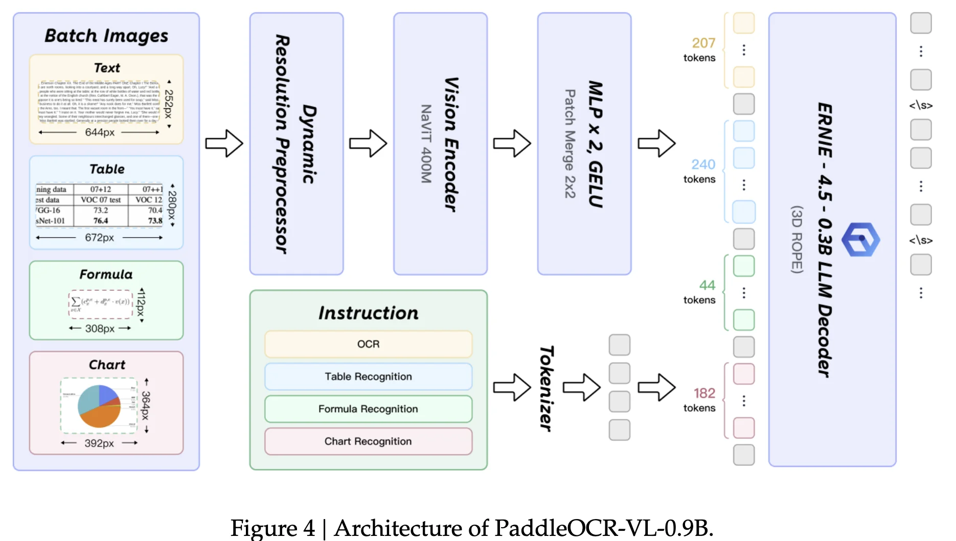
PaddleOCR-VL: Two-Stage Document Parsing with a 0.9B VLM
TL;DR
PaddleOCR-VL is a two-stage document parsing system: a lightweight layout analyzer (detect + reading order) followed by a 0.9B VLM (NaViT-style dynamic-resolution visual encoder + ERNIE-4.5-0.3B LM) that recognizes text, tables (OTSL), formulas (LaTeX), and charts (Markdown tables) across 109 languages. It posts SOTA/near-SOTA on OmniDocBench v1.0/v1.5 and olmOCR-Bench, while keeping inference lean via multithreaded, batched pipelines. Compared with end-to-end OCR VLMs, the decoupled layout stage improves reading-order stability, latency, and resource use.
What kind of paper is this?
- Dominant: $\Psi_{\text{Method}}$ (new system decomposition + VLM architecture choices + training recipe).
- Secondary: $\Psi_{\text{Resource}}$ (large-scale data construction pipeline with 30M+ samples across multiple synthesized/auto-labeled corpora).
- Also present: $\Psi_{\text{Evaluation}}$ (explicit throughput/VRAM benchmarking; inference efficiency comparisons across hardware).
What is the motivation?
- Document parsing needs layout understanding + reading order + element extraction (text/tables/formulas/charts) to support downstream retrieval and RAG workflows.
- The paper frames a tradeoff:
- Pipeline systems: strong but complex integration and error propagation.
- End-to-end VLM conversion: simpler interface but suffers from reading-order issues, hallucinations, and long-sequence latency/memory costs.
- Goal: get the stability benefits of pipelines with the simplicity of a compact VLM for element recognition.
What is the novelty?
- Two-stage decomposition: PP-DocLayoutV2 handles layout detection + reading order; PaddleOCR-VL-0.9B recognizes each cropped element. Outputs merge into structured Markdown + JSON.
- Decoupled reading order: RT-DETR + pointer network before VLM decoding mitigates long-context autoregressive burden and stabilizes ordering (a common failure mode in end-to-end VLM OCR).
- NaViT-style native dynamic resolution: fewer hallucinations on dense pages vs. fixed-size or heavy tiling; preserves aspect ratio without extreme token counts.
- 0.9B “ultra-compact” VLM: 0.3B decoder + strong visual encoder yields favorable accuracy/latency balance for production.
- Data engine: loops LLM-refined labels and typed hard-case synthesis to target weaknesses with measurable metrics.
Contrast with DeepSeek-OCR: DeepSeek uses SAM $\rightarrow$ conv-compressor $\rightarrow$ CLIP DeepEncoder to shrink tokens 16$\times$ and studies text/vision token ratios ($\approx$97% OCR at $\sim$10$\times$ compression). PaddleOCR-VL instead optimizes robustness + throughput under a document-parsing workflow with explicit reading order.
What experiments were performed?
- Page-level parsing: OmniDocBench v1.5 (1,355 pages), OmniDocBench v1.0 (981 pages), olmOCR-Bench; comparisons against pipeline tools, general VLMs, and specialized OCR VLMs.
- Element-level recognition:
- Text: OmniDocBench-OCR-block (17,148 crops) + in-house OCR set (107,452 line-level samples) + Ocean-OCR-Handwritten.
- Tables: OmniDocBench-Table-block (512 crops) + in-house benchmark (20 table types).
- Formulas: OmniDocBench-Formula-block (1,050 crops) + in-house benchmark (34,816 samples).
- Charts: in-house benchmark (1,801 samples) evaluated with RMS-F1.
- Inference/efficiency: end-to-end speed on OmniDocBench v1.0 (512 PDFs, A100), reporting pages/s, tokens/s, VRAM; cross-hardware configs (A10, RTX 3060/5070/4090D).
What are the outcomes/limitations?
Outcomes:
- OmniDocBench v1.5: overall 92.56; text edit distance 0.035; formula CDM 91.43; table TEDS 89.76; reading-order ED 0.043.
- olmOCR-Bench: overall 80.0 $\pm$ 1.0 unit-test pass rate (best), leading in ArXiv and Headers/Footers.
- Element-level wins across text/table/formula/chart benchmarks with detailed multilingual breakdowns.
- Throughput: 1.224 pages/s on A100 (+15.8% vs. MinerU2.5); ~43.7 GB VRAM (vs. dots.ocr ~78.5 GB).
Limitations:
- Reproducibility constraints: multiple critical components depend on in-house datasets and proprietary annotators (ERNIE-4.5-VL family); exact replication is difficult without equivalents.
- Coupling to detector quality: overall fidelity and order depend on RT-DETR + pointer network; OOD layouts may degrade.
- Less emphasis on token-economy: no explicit vision-tokens-per-page vs. accuracy frontier like DeepSeek-OCR.
- Output format assumptions: tables trained to OTSL, charts to Markdown tables, formulas to LaTeX; downstream consumers may need adapters.
- Charts grounding: strong RMS-F1 in-house, but public chart test sets are noisy/imbalanced.
Model
High-level architecture (Figures 2–4, pp.5–6)
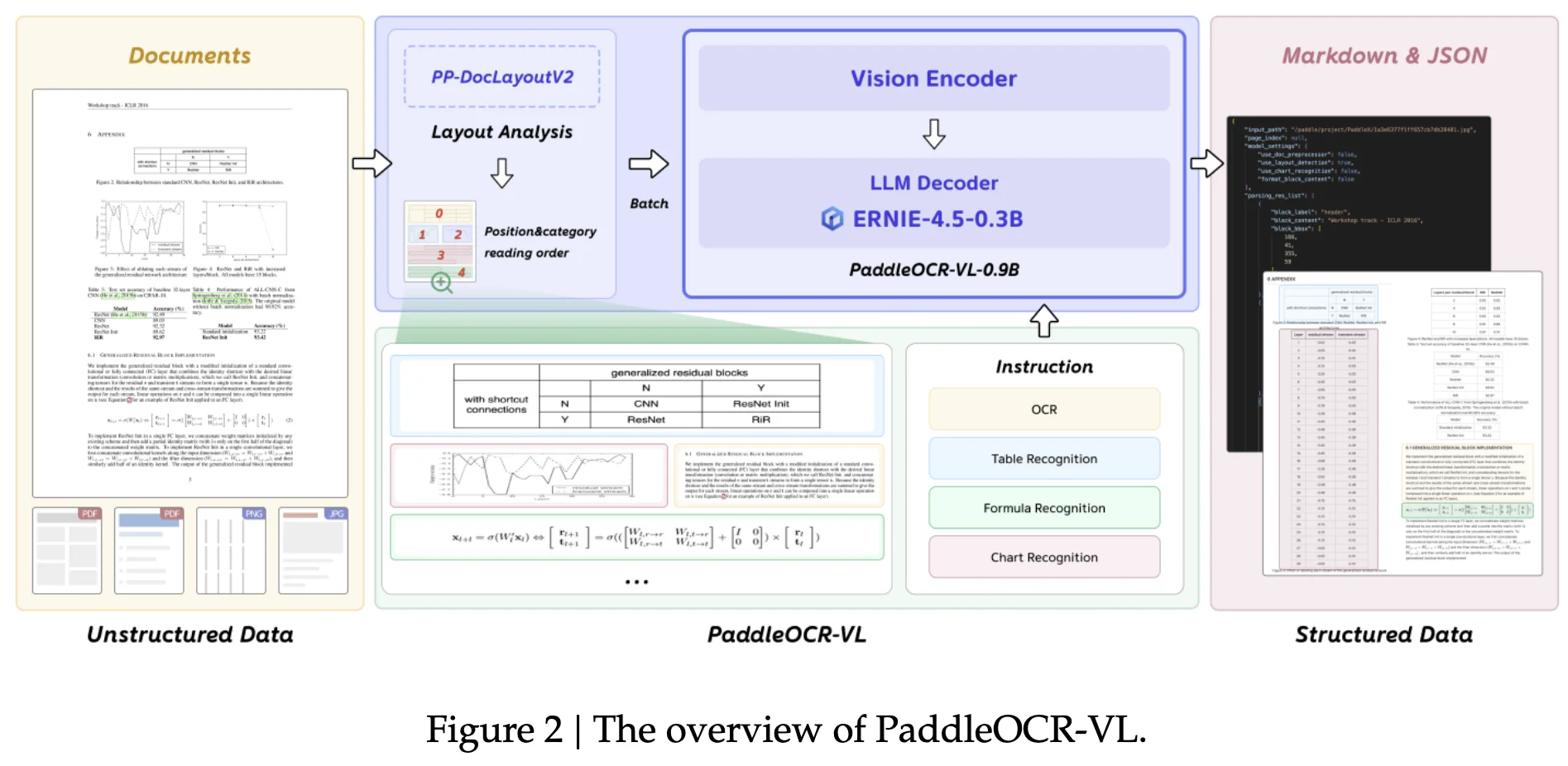
Two stages:
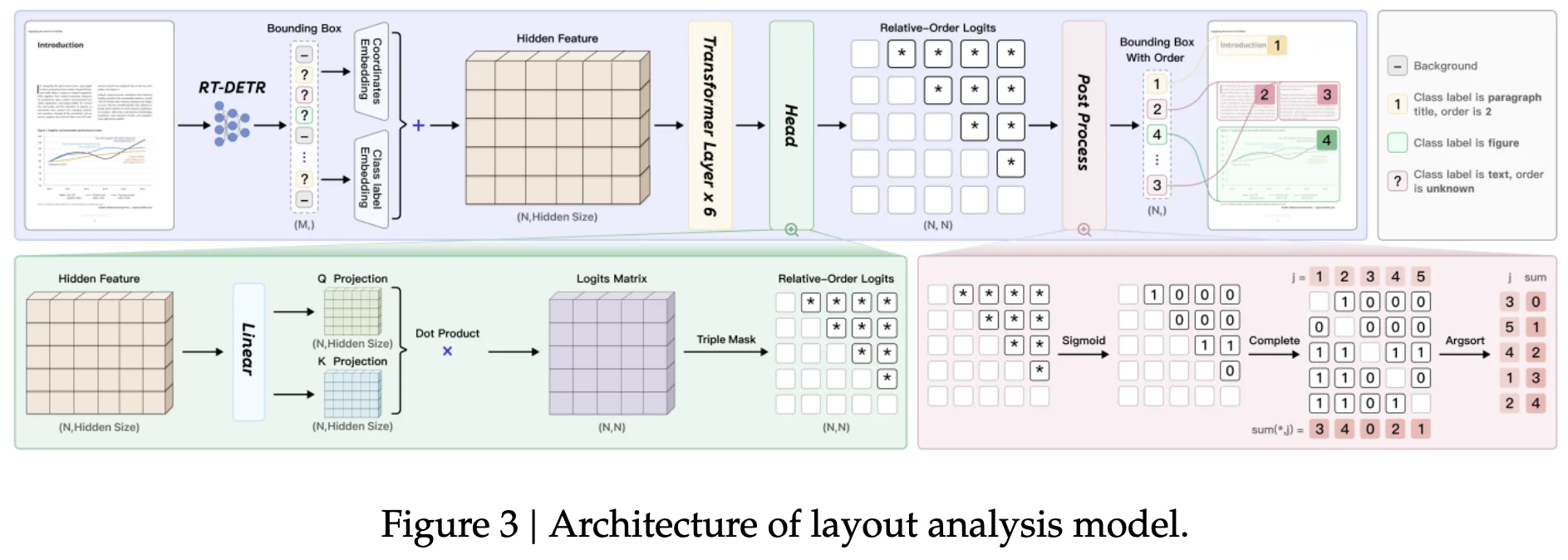
- PP-DocLayoutV2 (layout + reading order):
- Detector: RT-DETR for element boxes/classes (text blocks, tables, formulas, charts).
- Pointer network (6-layer Transformer) infers reading order: predicts an $N \times N$ pairwise order matrix using absolute 2D position encodings, class embeddings, and a geometry-biased attention head (Relation-DETR-style); decoded via deterministic win-accumulation to recover a topologically consistent ordering.
- Rationale: avoids end-to-end VLM hallucinations and long-sequence overhead for layout; keeps this step small and fast.
- PaddleOCR-VL-0.9B (element-level recognition):
- NaViT-style dynamic-resolution visual encoder (from Keye-VL), so it digests native-resolution crops without tiling distortion.
- 2-layer MLP projector (GELU; merge size 2).
- ERNIE-4.5-0.3B LM with 3D-RoPE as the text decoder (small decoder means faster AR decoding).
Design point vs. DeepSeek-OCR: PaddleOCR-VL decouples layout (specialized detector + ordering) from recognition, whereas DeepSeek-OCR is an end-to-end encoder–decoder optimized for optical compression of long text into few vision tokens. The former trades some end-to-end elegance for stability, lower latency, and cheaper training; the latter explores token-economy limits via compression.
“What the VLM emits”
- Text OCR: block/line/word-level transcription.
- Tables: OTSL structural tokens + content.
- Formulas: LaTeX (distinguishes inline
\(...\)vs. display\[...\]). - Charts: normalized Markdown tables.
Algorithms / Training (Section 2.2; Table 1, p.8)
- Layout (PP-DocLayoutV2):
- Train RT-DETR first (100 epochs on ~20k curated layout pages), then freeze it and train the pointer network for order (200 epochs; AdamW; GCE loss for noisy labels).
- VLM (PaddleOCR-VL-0.9B): two stages, all components trainable (ERNIEKit); batch size 128, sequence length 16,384 for both stages.
- Stage-1 alignment: 29M image–text pairs, max res $1280 \times 28 \times 28$ (NaViT), LR $5 \times 10^{-5} \rightarrow 5 \times 10^{-6}$, 1 epoch.
- Stage-2 instruction FT: 2.7M carefully curated samples, max res $2048 \times 28 \times 28$, LR $5 \times 10^{-6} \rightarrow 5 \times 10^{-7}$, 2 epochs; teaches 4 task families (OCR/table/formula/chart).
Data (Section 3; Figure 5, p.9)
Scale: 30M+ training samples across open datasets, synthesis, web-harvested documents, and in-house sets.
Three pillars:
- Curation from open sets (CASIA-HWDB, UniMER-1M, MathWriting; chart corpora like ChartQA/PlotQA/UniChart/Beagle/ChartINFO/visText/ExcelChart), synthesized data, web-scale crawl, and in-house corpora spanning many doc genres.
- Automatic annotation: PP-StructureV3 pseudo-labels $\rightarrow$ prompt LLMs (ERNIE-4.5-VL, Qwen2.5-VL) for refinement $\rightarrow$ hallucination filtering.
- Hard-case mining: build typed eval engines (23 text categories, 20 table types, 4 formula types, 11 chart families), score with EditDist, TEDS, CDM, RMS-F1 to find failures, then synthesize targeted data (XeLaTeX, web renderers). Reported synthesis rate: ~10,000 samples/hour for tables alone.
Hardware / Inference (Section 4.3; Table 13, p.18)
- Pipeline: three asynchronous threads (1) page rendering, (2) layout model, (3) batched VLM connected by queues; VLM batching triggers by queue size or dwell-time. vLLM/SGLang backends; knobs for max-batched-tokens and GPU memory utilization.
- Throughput (A100, vLLM, OmniDocBench v1.0):
- Pages/s: 1.224 (vs. MinerU2.5 1.057; +15.8%).
- Tokens/s: 1881 (vs. 1648; +14.2%).
- VRAM: ~43.7 GB; significantly less than dots.ocr (~78.5 GB) while being faster.
- Cross-hardware benchmarks also provided for A10, RTX 3060, RTX 5070, and RTX 4090D.
Evaluation
Page-level (full pages; Figures 1, Tables 2–3)
- OmniDocBench v1.5 — Overall 92.56; Text-Edit 0.035; Formula-CDM 91.43; Table-TEDS 89.76 / TEDS-S 93.52; Reading-Order ED 0.043. Top overall against pipelines and large VLMs.
- OmniDocBench v1.0 — Avg Overall-Edit 0.115; Text-Edit: EN 0.041, ZH 0.062; Table-TEDS: EN 88.0, ZH 92.1; Reading-Order ED: EN 0.045, ZH 0.063.
- olmOCR-Bench — Overall 80.0 $\pm$ 1.0 (best), leading in ArXiv and Headers/Footers; strong on Multi-column and Long tiny text.
Element-level (cropped blocks)
- Text (OmniDocBench-OCR-block) — lowest Edit Distance across most doc types (e.g., PPT2PDF 0.049, Academic 0.021, Newspaper 0.034).
- Handwriting (Ocean-OCR-Bench) — EN ED 0.118, ZH ED 0.034; best F1/Precision/Recall/BLEU/METEOR among compared systems.
- Tables (OmniDocBench-Table-block) — TEDS 0.9195, TEDS-struct 0.9543, Overall-ED 0.0561 (best).
- Formulas (v1.5 Formula-block) — CDM 0.9453; In-house formulas CDM 0.9882.
- Charts (in-house) — RMS-F1 0.844 overall, surpassing several specialized OCR VLMs and some 72B-scale VLMs.
Additional Notes
- Typed hard-case mining loop: the paper’s bucketed eval sets + targeted synthesis approach is a well-documented methodology for iterative data improvement.
- Prompting surface (Stage-2 tasks): the VLM is trained on four task families with distinct output formats:
- OCR: block/line/word transcription
- Tables: OTSL structural markup
- Formulas: LaTeX (inline vs. display)
- Charts: Markdown tables
- Contrast with DeepSeek-OCR: represents different design priorities; DeepSeek-OCR explores token-economy limits via optical compression ($\sim$97% OCR at $\sim$10$\times$ compression), while PaddleOCR-VL prioritizes robustness and throughput via decoupled layout.
olmOCR 2: Unit Test Rewards for Document OCR
TL;DR
olmOCR 2 is an OCR system built around a 7B VLM (Qwen2.5-VL-7B-Instruct base) trained with reinforcement learning using verifiable rewards (RLVR), where rewards come from a suite of binary unit tests. The authors scale unit-test creation by generating synthetic document pages with ground-truth HTML and extracted test cases, then apply GRPO-based RL to improve performance. They report an overall olmOCR-Bench score of 82.4 $\pm$ 1.1, a +14.2 point improvement over the initial olmOCR release, with large gains in math/table/multi-column handling.
What kind of paper is this?
Primarily $\Psi_{\text{Method}}$, with substantial $\Psi_{\text{Resource}}$ and $\Psi_{\text{Evaluation}}$ components.
- Dominant: $\Psi_{\text{Method}}$: The center of gravity is the training recipe (synthetic unit-test generation + GRPO RLVR) and the inference/system changes driving benchmark gains.
- Secondary: $\Psi_{\text{Resource}}$: The authors explicitly emphasize releasing model/data/code under permissive open licenses.
- Secondary: $\Psi_{\text{Evaluation}}$: A core argument is why binary unit tests can be preferable to edit distance for OCR correctness, supported by Figures 1–2 (p.3).
A rough superposition: 0.50 $\Psi_{\text{Method}}$ + 0.30 $\Psi_{\text{Resource}}$ + 0.20 $\Psi_{\text{Evaluation}}$.
What is the motivation?
- Need for clean, naturally ordered text from PDFs: The target is digitized print documents (like PDFs) converted into “clean, naturally ordered plain text.”
- Manual unit tests do not scale: The original olmOCR-Bench unit tests were manually verified and “took hours of work” to create/check, which blocks RL scaling.
- Edit distance is a weak proxy for OCR correctness in key cases:
- Floating elements lead to “ties” (multiple equivalent linearizations) that unit tests can treat equivalently, but edit distance can reward/penalize arbitrarily (Figure 1, p.3).
- Continuous scores can miss what matters: reading order vs caption placement; rendered correctness of equations vs LaTeX string similarity (Figure 2, p.3).
- Goal: Build a scalable pipeline where OCR outputs can be automatically verified via unit tests, enabling RLVR training at scale.
What is the novelty?
The paper combines and operationalizes several ideas into a cohesive training loop:
- Binary unit tests as verifiable RL rewards: Rewards are a “diverse set of binary unit tests” used for RLVR, rather than using only continuous text similarity.
- Synthetic pipeline to generate unit tests at scale: They create synthetic documents with known ground-truth HTML source and extracted test cases, enabling programmatic unit-test creation.
- Iterative PDF-to-HTML generation via a general VLM (Figure 3, p.4): They sample a real page and prompt a general VLM (
claude-sonnet-4-20250514) to produce a highly similar HTML page; the rendered HTML image paired with raw HTML becomes supervision. - GRPO-based RLVR on OCR: They apply Group Relative Policy Optimization (GRPO) using unit tests as binary reward signals.
- System/inference engineering that matters for OCR: Dynamic temperature scaling to avoid repetition loops, prompt-order standardization, YAML output format changes, and image resizing changes are described as meaningful contributors.
Contrast to Infinity Parser: The authors describe Infinity Parser as the closest related work; their stated key difference is binary unit tests as rewards vs Infinity Parser’s reward based on edit distance/paragraph count/structural consistency, plus differences in how real content seeds HTML generation.
What experiments were performed?
- Benchmarking on olmOCR-Bench (English): The benchmark measures unit-test types including:
- Text presence/absence, natural reading order, table accuracy, math formula accuracy via KaTeX rendering, baseline robustness.
- Comparisons vs other OCR systems (Table 1, p.2): They list multiple baselines (API-only, open-source, and VLM-based OCR systems), and report olmOCR 2 at 82.4 $\pm$ 1.1. The table caption notes their reproduction policy: results are reproduced in-house except those marked with
*. - Ablation-style incremental development breakdown (Table 3, p.7): They show stepwise improvements from “olmOCR (first release)” to “Synth data, RLVR, souping” and the resulting overall score changes.
- SFT dataset refresh comparison (Table 2, p.5): One-epoch finetuning on
olmOCR-mix-0225vsolmOCR-mix-1025with per-slice benchmark scores and overall results. - Metric motivation experiments (Figures 1–2, p.3):
- Figure 1: unit test vs edit distance for reading order errors with floating caption; unit tests treat valid placements as ties while edit distance penalizes some ordering choices more than others.
- Figure 2: unit test vs edit distance for math parsing; rendering-based checks can pass outputs with worse LaTeX edit distance and fail outputs with better edit distance.
What are the outcomes/limitations?
Outcomes reported:
- Overall improvement: +14.2 point improvement over the initial release when evaluated on the latest olmOCR-Bench, moving from 68.2 to 82.4.
- Where gains concentrate: The largest improvements are in math formula conversion, table parsing, and multi-column layouts.
- Open artifacts: Model/data/code released under permissive open licenses. Table 1 is structured to emphasize openness across model weights/training data/training code/inference code.
Limitations and open questions:
- Comparisons are heterogeneous: Table 1 includes systems with scores marked
*(reported by authors, not reproduced by the olmOCR team) and some entries show “$\pm$ ?” uncertainty, so “best overall” claims depend on which subset you view as comparable. - Benchmark scope: The benchmark is explicitly described as English-language; generalization beyond that is not established in this report.
- Unit-test coverage is a bottleneck: Any unit-test regime is inherently limited to the properties it encodes (a general risk for test-suite-based rewards). The authors explicitly want to extend the synthetic pipeline to more complicated document types/unit tests.
- Reliance on frontier model tooling in the pipeline: Synthetic generation uses
claude-sonnet-4-20250514, and the refreshed SFT mix is processed using GPT-4.1; reproducing the pipeline end-to-end may require access to these systems. - Binary vs continuous metrics: The paper argues binary tests often align better with correctness; still, calibrated continuous scores for non-math targets remain open work.
Model
Core model
olmOCR-2-7B-1025: A specialized 7B vision-language model trained with RLVR.- Base family: Starts from
Qwen2.5-VL-7B-Instructfine-tuned onolmOCR-mix-1025. The authors explicitly note switching from Qwen 2 VL to Qwen 2.5 VL for a slight benchmark gain. - FP8 variant:
olmOCR-2-7B-1025-FP8also released.
Output format and schema constraints
- Switched from JSON to YAML: To reduce retries; the authors speculate YAML avoids quote-count bookkeeping and reduces repetition loops.
- Document metadata at top: A reward term enforces that model outputs document metadata at the top (examples given: primary language, rotation correction factor).
Inference engineering (Section 4)
The authors highlight several system changes that materially affect end quality:
- Dynamic temperature scaling: Start at 0.1 and increase stepwise (0.2, 0.3, …) up to max 0.8 when EOS is not produced (to prevent repetition loops).
- Prompt ordering: Fix mismatch between training and inference prompt order by always placing text first; authors report improved performance and note this enables prompt caching.
- Image resizing: Increase from 1024 px to 1288 px on longest edge; authors describe this as a chosen balance between score and inference speed.
- Blank-page handling: Fix data loader skipping blank pages that caused hallucinations; no benchmark impact reported.
Contrast to DeepSeek-OCR: DeepSeek quantifies a frontier of 97% OCR at ~10$\times$ text$\rightarrow$vision compression with a SAM$\rightarrow$conv-16$\times$$\rightarrow$CLIP DeepEncoder (and token-economical multi-res modes), whereas olmOCR 2 largely keeps model size fixed and improves policy quality via unit-test rewards.
Data
Supervised fine-tuning (SFT) data: olmOCR-mix-1025
- Size: 267,962 pages from over 100,000 PDFs, including 9,828 pages from national archives.
- Delta vs previous mix (
olmOCR-mix-0225): Reprocessed using GPT-4.1 instead of GPT-4o; more consistent equation formatting using\[ ... \]and\( ... \); tables in HTML format; basic alt text for images.
Synthetic RL data: olmOCR2-synthmix-1025
- Size: 2,186 PDF pages with 30,381 unit test cases.
- Sourcing strategy: Sample real documents with “relevant, difficult-to-OCR material,” including arXiv math-heavy papers for equation-focused tests.
- General VLM used for HTML generation:
claude-sonnet-4-20250514. - Cost: Approximately $0.12 per document page (for the synthetic pipeline).
- Hallucination robustness claim: Pipeline is robust to Claude OCR errors because unit tests are generated from the HTML output alone.
Unit-test families
- Text presence/absence
- Natural reading order
- Table cell position
- Formula rendering (DOM/KaTeX)
- Baseline robustness (repeated n-grams, non-target language characters)
Algorithms / Training
Pipeline overview
The authors describe a two-part training recipe: (1) build a synthetic pipeline that renders documents into clean HTML and produces verifiable unit tests, then (2) apply GRPO to train using these binary reward signals.
Synthetic PDF-to-HTML generation steps
They break conversion into three steps (Figure 3, p.4):
- Layout analysis: Prompt a general VLM to describe layout (columns, images/tables, headers/footers) to guide HTML generation.
- Content rendering: Prompt again to “render this document as clean, semantic HTML” within original dimensions.
- Output refinement: Render generated HTML to an image, then prompt the VLM to refine HTML to better match the original image.
Unit test creation from HTML semantics
- Header/footer tags: By requiring
<header>and<footer>in HTML, they can generate “Text Absence” tests for those elements. - Math: Equations are rendered with KaTeX, enabling extraction and test creation for formula correctness.
- Tables: Extracted from ground truth; random cells sampled to create position/structure tests.
RLVR training details
- Base: Qwen2.5-VL-7B-Instruct fine-tuned on
olmOCR-mix-1025. - RL epoch: One epoch of RL training on
olmOCR2-synthmix-1025. - Compute: 8$\times$H100 GPU node.
- Sampling policy: 28 completions generated per document.
- Reward definition:
- Each unit test is pass/fail; reward is the fraction of passing tests, ranging 0.0 to 1.0.
- Figure 4 example: 4 of 6 tests passing yields page-level reward 0.67.
- Additional format rewards:
- Binary reward for ending with EOS token.
- Reward (0 to 1) for including document metadata at the top of the response.
- Implementation library and regularization: Hugging Face TRL with KL divergence $\beta = 0.01$.
- Model souping: Train six models with different random seeds and average (“soup”) their weights. They further note using importance sampling at token level (3 runs) and sequence level (3 runs) in that set of six runs.
Evaluation
Benchmark properties (unit tests)
The paper reiterates that olmOCR-Bench uses unit tests that can check: text presence, text absence (headers/footers/page numbers), reading order, table accuracy, math formula accuracy via KaTeX rendering, and baseline robustness against repeated n-grams or non-target language characters.
Why unit tests vs edit distance (Figures 1–2)
- Reading order “ties” (Figure 1, p.3): Floating caption can be correct either before or after a passage; unit tests can score both as equivalent, while edit distance penalizes some valid placements and partially rewards some invalid ones.
- Math formula rendering (Figure 2, p.3): Visually equivalent renderings can matter more than LaTeX string similarity; model A can have worse edit distance but pass rendering-based unit test, and vice versa.
Key results
Table 1 (system-level comparison, p.2):
- olmOCR 2 overall: 82.4 $\pm$ 1.1
- olmOCR (first release) overall: 68.2 $\pm$ 1.1
- Nearby systems (some marked
*as reported by authors, not reproduced):- Chandra OCR 0.1.0: 83.1 $\pm$ 0.9
* - Infinity-Parser 7B: 82.5 $\pm$ ?
* - dots.OCR: 79.1 $\pm$ 1.0
* - PaddleOCR-VL: 80.0 $\pm$ 1.0
*
- Chandra OCR 0.1.0: 83.1 $\pm$ 0.9
- The table annotates openness/licenses; olmOCR 2 highlights being fully open (weights, data, code).
Table 3 (incremental development breakdown, overall column, p.7):
- First release: 68.2 $\pm$ 1.1
- Dynamic temperature scaling: 72.8 $\pm$ 1.2
- Better prompting: 75.8 $\pm$ 1.0
- New trainer, YAML, image resize, Qwen 2.5 VL: 78.5 $\pm$ 1.1
- Handle blank pages: 78.5 $\pm$ 1.1
- Synth data, RLVR, souping: 82.4 $\pm$ 1.1
Biggest gains come from the RLVR stage.
Table 2 (SFT-only comparison, p.5):
One epoch finetuning on olmOCR-mix-0225 vs olmOCR-mix-1025 yields overall 78.5 $\pm$ 1.1 vs 78.3 $\pm$ 1.2, with mix-1025 showing better table slice score (77.9 vs 72.9) but worse “ArXiv” slice score (70.8 vs 78.6).
Hardware / Production
- RL training compute: 8$\times$H100 node, one epoch on synthetic RL data.
- Synthetic pipeline cost: Approximately $0.12 per document page using Claude Sonnet 4, with the note that hallucinations in Claude OCR do not affect their unit-test generation because they rely on HTML outputs.
- Production/API mention (high level): The authors thank inference partners DeepInfra and Parasail for helping set up public API access, but the report does not give latency/throughput numbers.
DeepSeek-OCR: Optical Compression for Document Understanding
TL;DR
DeepSeek-OCR is a VLM that treats an image of text as a compression medium: an encoder (“DeepEncoder”) maps high-res document images into a small number of vision tokens, and a 3B MoE decoder reconstructs the text. The authors report $\approx 97\%$ OCR decoding precision when the text-token count is $\le 10\times$ the vision-token count, and $\approx 60\%$ at $\approx 20\times$ compression; on OmniDocBench it aims to be competitive while using relatively few vision tokens.
What kind of paper is this?
Dominant: $\Psi_{\text{Method}}$ (new encoder design + multi-resolution token budgeting + end-to-end OCR system). Secondary: $\Psi_{\text{Evaluation}}$ (compression study on Fox; benchmarking on OmniDocBench); $\Psi_{\text{Resource}}$ (code/weights released; curated OCR training data).
What is the motivation?
- Long-context LLM compute scales quadratically with sequence length, so “just feed more text” is expensive.
- A document image can represent many words, suggesting vision tokens could serve as a cheaper “compressed representation” of long text.
- Prior open-source VLM vision encoders (dual-tower, tiling, NaViT-style adaptive resolution) each have issues for this use case: deployment complexity, too many vision tokens, high activation memory, or long packed sequences.
What is the novelty?
- Contexts optical compression framing: treat OCR as a compression-decompression mapping between document pixels $\rightarrow$ small vision-token sequence $\rightarrow$ reconstructed text, and study how many vision tokens are “enough” for a given amount of text.
- DeepEncoder: serially connects a window-attention perception module (SAM-base) to a dense global-attention knowledge module (CLIP-large) using a $16\times$ token compressor so high-res inputs do not explode dense attention cost.
- Multi-resolution token modes (Tiny/Small/Base/Large + dynamic tiling modes “Gundam”) to vary token budgets and study compression ratios.
What experiments were performed?
- Vision-text compression study: Fox benchmark, English docs with 600–1300 tokenizer tokens; evaluate OCR precision under 64 or 100 vision tokens (Tiny/Small). Reports precision vs. compression ratio.
- OCR practical performance: OmniDocBench; compares edit distance across categories (English/Chinese; text/formula/table/order; and per-document-type breakdown) across multiple model modes (Tiny $\rightarrow$ Gundam-M). Includes comparisons to pipeline OCR systems and other end-to-end VLM OCR models.
- Qualitative “deep parsing” demos: secondary calls to parse charts, natural images, chemical formulas, and simple geometry with a unified prompt style.
What are the outcomes/limitations?
Outcomes (reported):
- Fox compression: within $\approx 10\times$ compression, decoding precision reaches $\approx 97\%$; around $\approx 20\times$ compression precision is still $\approx 60\%$.
- OmniDocBench: at 100 vision tokens, the model is reported to surpass GOT-OCR2.0 (which uses 256 tokens/page in their table); at higher token modes (400, <800), it approaches or beats stronger baselines while using fewer tokens than some competitors.
- The paper positions this as evidence that compact decoders can learn to reconstruct text from heavily compressed visual latents, and proposes this as a direction for long-context handling.
Limitations / caveats (explicit or strongly implied):
- Fox evaluation notes formatting mismatches between output and ground truth can understate “true” OCR accuracy (their prompt-output format may not match the benchmark exactly).
- Degradation beyond $\approx 10\times$ is attributed to (a) more complex layouts in longer docs and (b) blur at 512–640 resolutions. Their proposed “fix” for (a) is rendering text into a single layout page, and they frame (b) as related to intentional forgetting.
- They state there is no SFT stage, so the model is “not a chatbot” and some capabilities require completion-style prompts.
- Several future-eval items are explicitly left open (digital-optical text interleaved pretraining, needle-in-a-haystack testing).
Model
High-level architecture
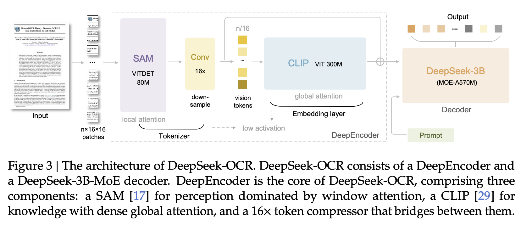
End-to-end VLM: DeepEncoder (encoder) + DeepSeek-3B-MoE (decoder).
DeepEncoder params: $\approx 380\text{M}$, composed of:
- SAM-base (patch size 16), $\approx 80\text{M}$ params, used as perception module dominated by window attention.
- CLIP-large, $\approx 300\text{M}$ params, used as knowledge module with dense global attention.
- A $16\times$ token compressor between them.
Decoder: DeepSeek-3B-MoE (routed MoE), 570M activated parameters at inference; activates 6 of 64 routed experts + 2 shared experts.
Token compressor details
Implemented as a 2-layer convolution module for $16\times$ downsampling of vision tokens:
- Each conv layer: kernel size 3, stride 2, padding 1.
- Channel increase: 256 $\rightarrow$ 1024.
Example: a 1024x1024 input yields $1024/16 \times 1024/16 = 4096$ patch tokens into the first stage; after the compressor, tokens reduce to $4096/16 = 256$ before dense global attention.
Why this design? The paper positions it between three common encoder families (dual-tower, tile-based, NaViT-style), avoiding their pitfalls (too many tokens, very low native resolution, huge activations):
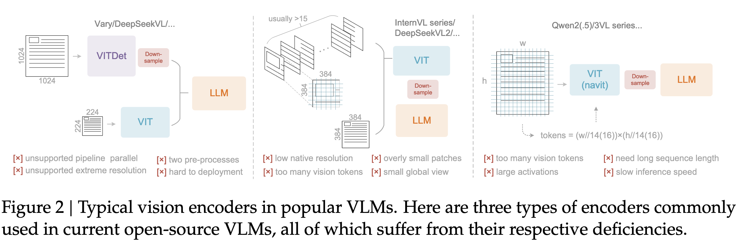
Multi-resolution modes and token budgets
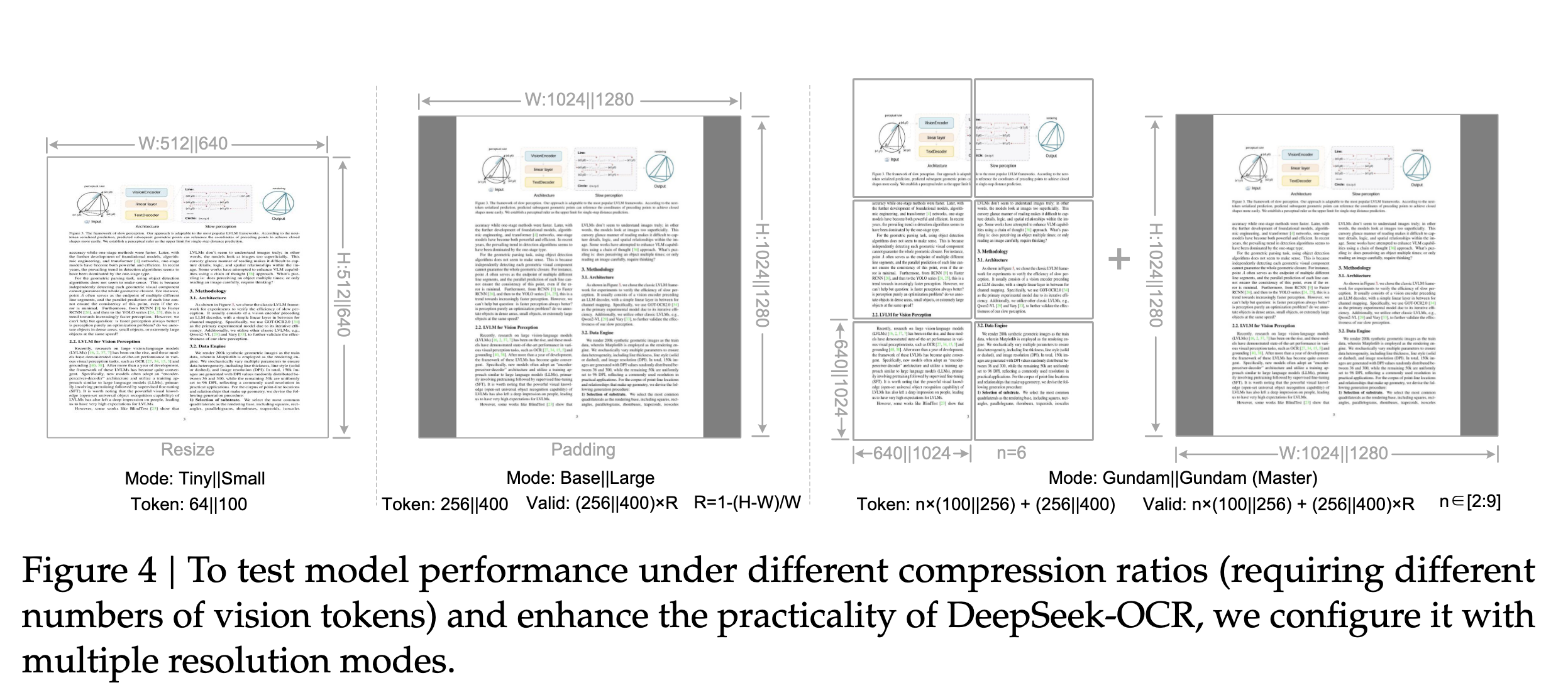
Native modes (single image, no tiling, fixed token budget):
- Tiny: $512 \times 512$ $\rightarrow$ 64 tokens (resize)
- Small: $640 \times 640$ $\rightarrow$ 100 tokens (resize)
- Base: $1024 \times 1024$ $\rightarrow$ 256 tokens (padding)
- Large: $1280 \times 1280$ $\rightarrow$ 400 tokens (padding)
Dynamic modes (global + tiles, variable token budget):
- Gundam: $n \times 640 \times 640$ tiles + $1024 \times 1024$ global $\rightarrow$ $n \times 100 + 256$ tokens, $n \in [2,9]$. If both sides $< 640$, it degrades to Base.
- Gundam-M: $n \times 1024 \times 1024$ tiles + $1280 \times 1280$ global $\rightarrow$ $n \times 256 + 400$ tokens (trained by continued training for load-balancing).
Positional encodings are dynamically interpolated to support all modes with a single model; tiling follows InternVL2.0.
For padded native modes, valid tokens:
$$N_{\text{valid}}=\left\lceil N_{\text{actual}}\times\left[1-\frac{\max(w,h)-\min(w,h)}{\max(w,h)}\right]\right\rceil$$
(Eq. 1).
Data
OCR 1.0 data (documents + scene text)
30M PDF pages across $\approx 100$ languages; Chinese+English $\approx 25\text{M}$ pages, other languages $\approx 5\text{M}$.
Two annotation types:
- Coarse annotations extracted via
fitzfor broad OCR coverage, especially minority languages. - Fine annotations: 2M pages Chinese + 2M pages English, labeled using layout (PP-DocLayout) + OCR systems (MinerU, GOT-OCR2.0) to create detection+recognition interleaved ground truth; for minority languages they describe a “model flywheel” using patch OCR to label patches after layout processing, producing 600K samples.
- Coarse annotations extracted via
3M Word documents: extract content to create high-quality image-text pairs (notably helpful for formulas and HTML tables).
Natural scene OCR:
- Sources: LAION, Wukong; labels via PaddleOCR.
- 10M Chinese + 10M English samples.
- Prompts can control whether detection boxes are output.
OCR 2.0 data (charts, chemistry, geometry)
- Charts: 10M rendered images (pyecharts + matplotlib); labels are HTML tables (explicitly not OneChart dictionary format) to save tokens.
- Chemical formulas: 5M image-text pairs; source SMILES from PubChem; render via RDKit; output target is SMILES.
- Plane geometry: 1M samples; generation follows “Slow Perception”; uses a perception ruler size of 4 per line segment; includes translation-invariant augmentation.
General vision + text-only mix
- General vision data for caption/detection/grounding is included to preserve a general vision interface; authors state it is 20% of training data.
- Text-only pretraining data is 10%, processed to 8192 tokens (also the full model sequence length).
- Overall mix: 70% OCR, 20% general vision, 10% text-only.
Algorithms / Training
Stage A: Train DeepEncoder
- Objective: next-token prediction using a compact language model, following Vary-style training.
- Data: all OCR 1.0 + OCR 2.0 + 100M general samples from LAION.
- Training: 2 epochs, batch size 1280, AdamW, cosine annealing, learning rate $5\times10^{-5}$, sequence length 4096.
Stage B: Train full DeepSeek-OCR
Platform: HAI-LLM.
Pipeline parallelism: 4 partitions:
- PP0: SAM + compressor as “vision tokenizer”, frozen.
- PP1: CLIP part as embedding layer, unfrozen.
- PP2/PP3: DeepSeek3B-MoE has 12 layers, split 6 + 6.
Compute: 20 nodes, each 8x A100-40G; DP=40; global batch size 640.
Optimizer/schedule: AdamW, step-based scheduler, initial LR $3\times10^{-5}$.
Throughput: text-only $\approx 90\text{B}$ tokens/day; multimodal $\approx 70\text{B}$ tokens/day.
Gundam-M is trained via continued training on a trained model (they cite load balancing / speed issues if trained jointly).
Prompts / interfaces (examples shown in paper)
<image>
Free OCR.

<image>
<|grounding|>Convert the document to markdown.

<image>
Parse the figure.
(These are used to control layout output and deep parsing behavior.)
Hardware / Production
Data-generation throughput claims:
- Abstract: “200k+ pages per day” on a single A100-40G.
- Intro: “33 million pages per day” using 20 nodes (each 8x A100-40G).
The paper frames “contexts optical compression” as enabling a forgetting-like mechanism: render older dialogue rounds into images and progressively downsize them so older context gets blurrier and cheaper (Figure 13).
Evaluation
Fox benchmark: compression ratio vs precision
Setup: English Fox docs, ground-truth tokens 600–1300 (using DeepSeek-OCR tokenizer, vocab size $\approx 129\text{k}$), 100 pages; evaluate Tiny (64) and Small (100) modes.
Reported table highlights (precision, compression):
- 600–700 tokens: 64 toks $\rightarrow$ 96.5% at 10.5$\times$; 100 toks $\rightarrow$ 98.5% at 6.7$\times$
- 1200–1300 tokens: 64 toks $\rightarrow$ 59.1% at 19.7$\times$; 100 toks $\rightarrow$ 87.1% at 12.6$\times$
OmniDocBench: edit distance vs tokens
Metric: edit distance (lower is better), across English/Chinese and subcategories (text/formula/table/order), plus overall; “Tokens” is avg vision tokens per page, with parentheses indicating “valid” tokens for padded modes.
DeepSeek-OCR modes (tokens shown as reported):
- Tiny: 64
- Small: 100
- Base: 256 (182 valid)
- Large: 400 (285 valid)
- Gundam: 795
- Gundam-M @200dpi: 1853
Document-type breakdown suggests some categories (slides, books, reports) work well with low tokens, while newspapers require Gundam-class modes due to much higher text-token counts (4–5k).
POINTS-Reader: Distillation-Free Document Conversion via Iterative Self-Improvement
TL;DR
POINTS-Reader is a 4B-parameter document-conversion VLM built on POINTS-1.5 and trained via a two-stage, distillation-free pipeline: synthetic “uniform format” warm-up (800K samples across plain text, formulas, tables, multi-column layouts) and iterative self-improvement on real PDFs (DocMatix) with rule-based filtering. By unifying outputs for text (Markdown), tables (HTML), and formulas (LaTeX) and repeatedly bootstrapping on its own filtered annotations, the model surpasses many larger VLMs and OCR experts on OmniDocBench and Fox, especially for tables, while still trailing pipeline systems like MinerU and Mathpix.
What kind of paper is this?
Dominant: $\Psi_{\text{Method}}$ (training procedure: synthetic warm-up plus iterative self-improvement with rule-based filtering, rather than new architecture).
Secondary: $\Psi_{\text{Resource}}$ (implicitly releases carefully filtered HTML-table, formula-aware dataset of $\sim$1.1M high-quality samples plus trained model); $\Psi_{\text{Evaluation}}$ (ablations on data scale, aspect ratio filtering, F1 thresholds, sampling ratios, initialization choices, all quantified on OmniDocBench).
The core contribution is a training methodology that avoids distillation from proprietary or very large models. The paper demonstrates that careful synthetic data design plus iterative bootstrapping with strict automated quality filters can produce competitive document-conversion models without inheriting teacher model biases or errors.
What is the motivation?
High-quality labeled data for end-to-end document conversion (text plus tables plus math plus layout) is scarce and expensive to annotate. Existing approaches usually distill from proprietary or very large open VLMs (GPT-4o, Qwen2.5-VL-72B, etc.), which locks progress to teacher capabilities and transfers teacher errors and biases (missing tables, hallucinated or omitted text, wrong table structure). Purely synthetic data helps but diverges from real-world layouts; models trained only on synthetic images underperform on complex PDFs. The goal is to learn a strong OCR/VLM reader without distillation by warm-starting on synthetic but layout-diverse data with unified output format, then adapting to real documents via self-improvement on DocMatix with strict automated filtering.
What is the novelty?
Unified output representation for document elements:
- Plain text: standardized Markdown (headers, lists, etc.)
- Tables: HTML
<table>with simplified attributes, no CSS except merged-cell info, no extra whitespace or indentation to keep tokens down - Formulas: KaTeX-compatible LaTeX,
$...$inline and$$...$$display
Two-stage distillation-free training pipeline:
- Uniform Format Warm-up Stage (UWS): LLM-generated synthetic documents across four categories (plain text, text plus formulas, text plus tables, multi-column layouts with tables). HTML templates (1/2/3-column) rendered with headless Chrome to produce image–text pairs.
- Iterative Self-improvement Stage (ISS): Use the warm-up model to annotate millions of real DocMatix pages; filter predictions (plain-text F1 vs PaddleOCR, HTML structural checks for tables, syntax checks for LaTeX); retrain on filtered set; repeat for several iterations.
Rule-based data filtering at scale:
- Bag-of-words F1 against PaddleOCR for text
- Structural validation for tables
- Syntax validity for formulas
Empirical insights about data and training:
- Sweet spot in synthetic data size ($\sim$800K samples) beyond which performance drops due to distribution mismatch
- Restricting aspect ratio to $\sim[0.4, 2.5]$ removes pathological images and improves results
- Always re-initializing each iteration from the base pre-trained model (POINTS-1.5) is better than continuing from the previous iteration
- Including UWS data in later ISS iterations helps, despite its synthetic nature, because its annotations are very clean
What experiments were performed?
Warm-up ablations (OmniDocBench overall metric, lower is better):
- Incrementally adding each synthetic category (plain text, then plus formulas, then plus tables, then plus multi-column tables) while keeping 200K samples per category (800K total)
- Scaling total synthetic data from 100K to 1.2M to find saturation/overfitting point
- Filtering images by aspect ratio ranges to prune extreme shapes
Self-improvement ablations:
- Adding filters in stages (text, then table, then formula) and measuring improvements
- Sweeping F1 thresholds for text filtering (0.70, 0.80, 0.90, 0.95)
- Varying sampling ratios for plain text vs tables vs formulas during training
- Comparing initialization from previous iteration vs re-starting from the original POINTS-1.5 weights
- Tracking performance vs ISS iteration count (up to five rounds), with curves for OmniDocBench, global F1 vs PaddleOCR, and retained data volume
Dataset comparison:
- Compare the final distilled-free dataset ($\sim$1.1M samples) to KOSMOS-2.5 training data and olmOCR data (size, table format, distillation vs non-distillation, language coverage)
Baseline comparisons on OmniDocBench (en) and Fox-Page-en:
- Pipeline methods: MinerU, Marker, Mathpix
- General VLMs: Qwen2.5-VL (3B, 7B, 72B)
- Expert OCR/VLM: GOT-OCR, Nougat, Mistral OCR, OLMOCR
- Additionally: a version of POINTS-Reader trained directly on distillation data from Qwen2.5-VL-72B
What are the outcomes/limitations?
Outcomes (as reported):
On OmniDocBench (en):
- POINTS-Reader (4B) overall edit distance 0.259, beating several larger specialized and general models:
- Qwen2.5-VL-3B: 0.390; Qwen2.5-VL-7B: 0.331; GOT-OCR: 0.287; OLMOCR-7B: 0.326
- Particularly strong table performance: 0.335 vs 0.341 for Qwen2.5-VL-72B and much better than GOT-OCR on the same metric (gap $\approx 0.197$)
On Fox-Page-en (edit distance, lower is better):
- POINTS-Reader: 0.023, outperforming all listed general VLMs and OCR baselines in the table (e.g., Qwen2.5-VL-72B at 0.027)
Compared to a model directly distilled from Qwen2.5-VL-72B, the distillation-free POINTS-Reader is decisively better (overall 0.259 vs 0.302) on OmniDocBench.
However, pipeline systems like MinerU and Mathpix still achieve lower error overall than any end-to-end VLM, including POINTS-Reader, highlighting remaining performance gaps.
ISS curves show monotonic improvement across iterations on OmniDocBench, global F1 vs PaddleOCR rising from $\sim$0.70 up to $\sim$0.84, and number of retained filtered samples increasing for text, tables, and formulas over iterations.
Limitations (acknowledged by authors):
- Language: Training and evaluation are English-only; multi-lingual and CJK support are future work
- Content type: Datasets are largely printed fonts; performance on handwritten notes is suboptimal. The model currently extracts only plain text, formulas, and tables, not images or figure locations
- Data supervision: Table and formula filters check only structure and syntax, not semantic correctness, so some residual label noise remains
- Benchmark scope: Focus is on Fox and OmniDocBench; there is no evaluation on real production workflows or domain-specific documents (e.g., handwritten forms, multi-language PDFs)
Model
Backbone and overall architecture
- Base model: POINTS-1.5 VLM as the visual encoder plus multimodal connector
- Language backbone: Qwen2.5-3B-Instruct as the LLM head, chosen for efficiency vs quality trade-off
- Parameter scale: $\sim$4B parameters
- Context length: 8192 tokens in this work (longer than default POINTS-1.5)
- Training paradigm inherited from POINTS-1.5:
- Pretraining on generic vision–language data
- Visual instruction tuning (VIT) with both the synthetic UWS data and filtered ISS data, plus general data from POINTS-1.5
- All hyperparameters and settings except VIT data and context length are identical to POINTS-1.5, so this paper’s novelty sits almost entirely in the data and training pipeline rather than architecture tweaks
Input and output format
- Input: Document page images, often multi-column, with tables and formulas. Real data comes from PDF-derived PNGs in DocMatix
- Output: Single text sequence in the unified markup format:
- Plain text: Markdown headings, lists, bold/italic, etc.
- Tables: Minimal HTML table markup with no whitespace between tags, no CSS apart from merged-cell attributes; same format used for both synthetic and real annotations
- Formulas: LaTeX obeying KaTeX rules,
$...$inline,$$...$$display
Data
1. Uniform Format Warm-up (Synthetic)
Unified output format:
- Text: Markdown (following Kosmos-2.5 style choices)
- Tables: HTML to handle complex structures (merged cells) more flexibly than Markdown; LaTeX tables rejected due to non-standard and variable syntax
- Formulas: KaTeX-compatible LaTeX syntax
Generation pipeline:
- LLM text generation: Prompts instruct a large language model to generate document-like Markdown, including topic selection, 300–800 words depending on category, style choices from exam papers, slides, academic papers, books, textbooks, magazines, notes, newspapers, financial reports, and optional use of Markdown constructs (headings, lists, bold/italic, subscripts/superscripts). Formula-containing prompts encourage varied LaTeX constructs (matrices,
align,gather,frac,sum, etc.), mixing inline and display math. Multi-column prompts split content into two logical chunks separated by a marker string"x----------x"for later layout templating. - Category design: Four synthetic categories (plain text; text plus formulas; text plus tables, single-column; multi-column layouts with tables)
- Table enrichment: LLM-prompting alone tended to produce simple tables, so they augment with real tables from PubTabNet training set, generating descriptive paragraphs and then inserting those tables into the text at random positions
- Filtering (synthetic side): Apply the same LaTeX formula and HTML table filters as in ISS (syntax/structure checks) before rendering
- Rendering: Convert the unified text into HTML and render images with 1/2/3-column templates using Chrome headless mode
Synthetic dataset scale:
- For ablations: 200K filtered samples per category yields 800K total; this configuration gives the best performance
- Scaling from 100K to 1.2M samples shows gains up to $\sim$800K, then degradation (overfitting to synthetic layouts that diverge from real PDFs)
- Aspect ratio filtering: Inspect distribution of width/height and cut off extreme aspect ratios outside $[2/5, 5/2]$. This removes overly tall or wide renderings and measurably improves OmniDocBench scores
2. Iterative Self-improvement (Real Data)
Base real-world corpus:
- DocMatix: More than 2M images derived from PDF/A, covering academic papers, textbooks, exams, and various document types
- Total used: 2,234,134 images; in the final ISS iteration, $\sim$1.1M (1,096,325) pass filters and are used for training
Element distribution (final ISS iteration):
- Only plain text: 90.2% of samples
- Contains tables: 6.5%
- Contains formulas: 3.3% (about 0.1% have both tables and formulas)
Token length distribution:
- Most training samples are shorter than 1,000 tokens
Final dataset comparison:
| Dataset | Size | Tables Format | Distillation | Language |
|---|---|---|---|---|
| KOSMOS-2.5 | 357.4M | Markdown | Yes | English |
| olmOCR | 260K | Markdown | Yes (GPT-4o) | English |
| POINTS-Reader | $\sim$1.1M | HTML | No | English |
Algorithms and Training
1. Plain-text F1 filtering
For text quality control, they compare POINTS-Reader predictions to PaddleOCR outputs as pseudo-ground-truth:
- Normalize both prediction and reference strings (strip non-alphanumeric characters, split on spaces and count occurrences of each token)
- Let $P = {(u^p_i, c^p_i)}$ be prediction tokens and counts, $T = {(u^t_i, c^t_i)}$ be reference tokens and counts
- Define:
$$\text{Precision} = \frac{\sum_i \min(c^p_i, c^t_i)}{\sum_i c^p_i},\quad \text{Recall} = \frac{\sum_i \min(c^p_i, c^t_i)}{\sum_i c^t_i}$$
$$F_1 = \frac{2 \times \text{Precision} \times \text{Recall}}{\text{Precision} + \text{Recall}}$$
- Discard samples with $F_1$ below a threshold
Ablation on thresholds: 0.90 gives the best overall OmniDocBench score, balancing quality and coverage; 0.70 and 0.95 both hurt performance relative to 0.90.
2. Table filtering
They do not use external structure-recognition models as teachers, due to robustness issues and table-only assumptions. Instead, they parse each HTML table in the output and enforce structural validity:
- Consistent numbers of cells per row/column
- Valid merged-cell attributes
Samples with malformed table structures are dropped.
3. Formula filtering
- Extract all LaTeX formulas from the output and run syntax checks (KaTeX-compatible)
- Samples containing any syntactically invalid formula are discarded
- They explicitly do not check semantic correctness (e.g., whether the math equals the underlying document)
4. Iterative self-improvement loop
Each ISS iteration:
- Run the current model on the full DocMatix dataset to produce annotations (image to unified markup)
- Apply the three filters in order: text F1, table structure, formula syntax
- Use all retained image–text pairs to perform visual instruction tuning from the base POINTS-1.5 weights, not from the previous ISS iteration’s weights (this choice is empirically better)
- Include UWS synthetic data in ISS training; this reliably improves performance
Findings from ISS:
- Each iteration improves both OmniDocBench performance and DocMatix F1 vs PaddleOCR
- The volume of retained samples with text/tables/formulas grows per iteration, indicating the model is generating more usable annotations
- Improvements come from a combination of better original training data and increased diversity from new filtered samples
5. Sampling ratios
Because plain-text-only samples dominate, they tested aggressive rebalancing: lowering the plain-text sampling probability and up-weighting tables and formulas. This rebalancing hurts performance; best results come from sampling directly from the natural distribution (1.0:1.0:1.0 weights). Hypothesis: down-sampling text reduces diversity without increasing table/formula diversity (just repeats the same small set more often), degrading generalization.
Evaluation
Benchmarks and metrics
- OmniDocBench (English split): 19 layout types; evaluates text edit distance, formula edit distance, table edit distance, reading order correctness. Overall metric is a blend of these (all normalized edit distances; lower is better)
- Fox-Page-en (English split of Fox): 112 pages, single and double column, each with more than 1K words. Metric: normalized edit distance between model outputs and references; lower is better
Core comparisons
Pipeline methods (MinerU, Marker, Mathpix):
- Achieve the lowest OmniDocBench error overall; still the strongest approach for document conversion in this comparison
General VLMs:
- Qwen2.5-VL-72B is the strongest among generic models (overall $\sim$0.214) but much larger than POINTS-Reader
- Smaller Qwen2.5-VL (3B, 7B) lag behind POINTS-Reader on both OmniDocBench and Fox
Expert VLM/OCR:
- GOT-OCR, Nougat, Mistral OCR, OLMOCR all underperform relative to POINTS-Reader on the combined OmniDocBench metrics, especially for tables
- POINTS-Reader vs Mistral OCR: substantial gain in OmniDocBench overall (0.259 vs 0.268) and much better tables
Ablation highlights
| Experiment | Configuration | OmniDocBench Overall $\downarrow$ |
|---|---|---|
| Synthetic diversity | Plain text only | 0.626 |
| + Formulas | 0.579 | |
| + Tables | 0.538 | |
| + Multi-column tables | 0.510 | |
| Aspect ratio filtering | No filtering | 0.515 |
| $[2/5, 5/2]$ | 0.498 | |
| ISS filtering | No filters | 0.493 |
| + Text F1 filter | 0.463 | |
| + Table filter | 0.447 | |
| + Formula filter | 0.439 | |
| Distillation comparison | Distilled from Qwen2.5-VL-72B | 0.302 |
| POINTS-Reader ISS (no distill) | 0.259 |
Hardware and Production
- All experiments run on 64 $\times$ NVIDIA H800 GPUs
- Approximate costs reported:
- Training on 1M samples $\approx$ 7 hours
- Inference on 2M DocMatix images $\approx$ 10 hours using SGLang for deployment-time serving
- The paper does not detail batching strategies or peak throughput, but given the 4B parameter count and 8192-token context, the model is engineered to be relatively efficient compared to 70B-class VLMs, while still relying on a sizable GPU cluster for each self-improvement iteration
Note: This analysis follows the Roots Labs OCR paper-notes guidelines and classification taxonomy. For academic or production use, consult the original paper and verify claims through independent evaluation.
MinerU2.5: Coarse-to-Fine Document Parsing with Decoupled Layout
TL;DR
MinerU2.5 is a 1.2B-parameter vision language model for document parsing that decouples global layout analysis from local content recognition using a coarse-to-fine, two-stage inference pipeline (thumbnail layout first, then native-resolution crops). With a NaViT vision encoder (675M params), a Qwen2-0.5B decoder with M-RoPE, and a pixel-unshuffle patch merger, it achieves strong results on OmniDocBench (Overall 90.67) while maintaining practical throughput ($\approx$ 2.12 pages/s on A100-80G). The paper introduces PageIoU (layout metric), ADR (atomic decomposition for long formulas), OTSL (compact table target), and IMIC (consistency-based hard-case mining).
What kind of paper is this?
Primarily $\Psi_{\text{Method}}$ with strong $\Psi_{\text{Resource}}$ and $\Psi_{\text{Evaluation}}$ components.
The headline novelty is the two-stage decoupled parsing architecture: thumbnail-based layout detection followed by native-resolution crop recognition. Secondary contributions include new evaluation methodology (PageIoU metric) and a data flywheel (IMIC mining strategy). The model weights and code are publicly released.
Rough superposition: $\Psi_{\text{Method}}(0.65) + \Psi_{\text{Resource}}(0.20) + \Psi_{\text{Evaluation}}(0.15)$
What is the motivation?
High-resolution document parsing faces a fundamental tension: native-resolution processing yields better recognition quality but incurs $O(N^2)$ attention costs over massive token sequences. Existing solutions have critical gaps:
- Pipeline systems are modular but suffer from error propagation and cumbersome integration
- End-to-end VLMs are bottlenecked by hallucinations on long documents and token redundancy from blank or low-information regions
- Prior systems either sacrifice resolution (hurting small text/formulas) or sacrifice throughput (impractical for production)
MinerU2.5 addresses this by decoupling global layout from local content: make layout explicit in Stage I on a cheap thumbnail, then “spend” tokens only on content-bearing crops in Stage II at native resolution.
What is the novelty?
The core contribution is a coarse-to-fine, two-stage decoupled parsing architecture:
- Stage I (global): Predict layout/rotation/reading-order on a fixed 1036$\times$1036 thumbnail, avoiding native-resolution $O(N^2)$ token blowup
- Stage II (local): Process native-resolution crops independently, enabling parallelism and bounded token counts
Supporting innovations:
- PageIoU: A page-level coverage metric for layout using coverage maps and pixel-wise min/max aggregation, better matching human perception than IoU@0.5 for text blocks (Figure 4, p. 15)
- ADR (Atomic Decomposition & Recombination): For multi-line formulas, decompose into atomic lines, recognize each, then recombine with LaTeX alignment (Figure 5, p. 16)
- OTSL: A compact table representation reducing structural tokens from $\sim$28 to 5, shrinking sequences by $\sim$50% (Figure 6, p. 17)
- IMIC (Iterative Mining via Inference Consistency): Run stochastic decoding multiple times; low consistency (measured by PageIoU/TEDS/CDM) flags hard cases for human annotation (Figure 7, p. 18)
- M-RoPE: Replace 1D-RoPE with multi-dimensional RoPE to generalize across varying crop resolutions/aspect ratios
What experiments were performed?
Evaluation spans six benchmark categories with detailed ablations:
- Full-page parsing: OmniDocBench (1,355 pages, EN/ZH) measuring text edit distance, formula CDM, table TEDS/TEDS-S, reading order edit distance
- Dense text OCR: Ocean-OCR (EN/ZH splits) with edit distance, F1, BLEU, METEOR metrics
- Unit tests: olmOCR-bench (math, scans, tiny text) using ExpRate (render-based) for math splits instead of AST-string CDM
- Layout analysis: OmniDocBench, D4LA, DocLayNet using PageIoU metric with unified tag set (headers, footers, page numbers, code, algorithms, references, lists, caption sub-types)
- Table recognition: PubTabNet, FinTabNet, CC-OCR, OCRBench v2, in-house TR dataset
- Formula recognition: CPE, HWE, SCE, SPE, LaTeX-80MM, plus in-house Chinese/Fuzzy/Complex sets
Baselines include Qwen2.5-VL (7B/72B), InternVL3, Gemini-2.5-Pro, and specialized systems (GOT, Docling, MinerU2). The paper also provides throughput benchmarks across A100-80G, RTX 4090-48G, and H200-141G.
What are the outcomes/limitations?
Key results (Tables 5–11, pp. 19–24):
- OmniDocBench Overall: 90.67 (best reported), with Text-Edit 0.047, TEDS 88.22, CDM 88.46, RO-ED 0.044
- Overall score defined as: $\text{Overall} = \frac{(1-\text{TextEdit}) \times 100 + \text{TableTEDS} + \text{FormulaCDM}}{3}$
- FinTabNet: TEDS 95.97 / TEDS-S 97.61 (leading by margin)
- olmOCR-bench: 75.2 overall (best among listed); AR (math) 76.6, Old Scans Math 54.6, Long Tiny Text 83.5
- Ocean-OCR English: ED 0.033, F1 0.945, BLEU 0.909, METEOR 0.950
- Throughput: 2.12 pages/s (A100-80G), 4.47 pages/s (H200-141G), 1.70 pages/s (RTX 4090-48G) via vLLM
Limitations and open questions:
- Stage I is a recall bottleneck: Missed or merged elements in layout propagate to Stage II; the system cannot recover from layout errors
- Cross-domain robustness depends on the data engine: Rare layouts (multi-page wraps, exotic scripts) may require targeted IMIC mining
- Heuristic tuning: Crop scheduling and repetition penalties are manually tuned; learned scheduling policies could improve batch efficiency
- Dependency on frontier models: The data curation pipeline uses Qwen2.5-VL-72B, Gemini-2.5-Pro for pre-annotation, which may limit reproducibility
Model
Architecture (Figure 2, p. 7)
| Component | Details |
|---|---|
| Vision encoder | NaViT (Native-Res ViT), $\sim$675M params, 2D-RoPE, arbitrary aspect ratios |
| Patch merger | Pixel-unshuffle $2\times 2$, reduces vision tokens before LM |
| LM decoder | Qwen2-Instruct 0.5B with M-RoPE |
| Total | $\sim$1.2B params |
Key architectural choices:
- NaViT with 2D-RoPE: Chosen over Qwen2.5-VL’s window attention, which the authors note can degrade document parsing performance
- M-RoPE (multi-dimensional RoPE): Replaces 1D-RoPE in the LM decoder to generalize across varying crop resolutions and aspect ratios
- Pixel-unshuffle patch merger: Merges adjacent $2 \times 2$ vision tokens before feeding to the LM, trading off efficiency and performance
Two-stage pipeline
- Stage I (global layout):
- Input: Uniformly resized to 1036$\times$1036 pixels
- Output: Box positions, classes, rotation angles, and reading order in a single pass
- Benefit: Fixed thumbnail improves box stability and training efficiency
- Stage II (local content):
- Input: Crops from original high-res image using Stage I boxes
- Resolution: Native resolution with upper bound of 2048$\times$28$\times$28 pixels
- Output: Text, table (OTSL format), or formula (LaTeX) per crop
- Benefit: Crops process independently, enabling batching and parallelism
Task reformulations
Layout analysis as multi-task: Predict Position, Class, Rotation Angle, and Reading Order in one pass (instead of pushing rotation/order downstream to separate stages).
Formulas (ADR): “Whole-part” approach classifies formulas as atomic vs compound, decomposes compound formulas into lines, recognizes each line, then recombines using layout info.
Tables (OTSL): Generate OTSL instead of HTML to reduce structural token redundancy (structural tokens reduced from “over 28” down to “5”, $\sim$50% shorter sequences), then convert to HTML post-processing.
Prompts (Appendix B)
Task-specific prompts switch output format:
<image>
Layout Detection:
Output: box positions, classes, rotation, reading order tokens
<image>
Text Recognition:
Output: OCR Results:{text}
<image>
Formula Recognition:
Output: LaTeX:{latex}
<image>
Table Recognition:
Output: OTSL:{otsl}
Contrast to end-to-end OCR VLMs: Instead of attending over massive native-res token sequences for the whole page, MinerU2.5 filters with Stage I and only “spends” tokens on content-bearing crops. This cuts $O(N^2)$ token growth, reduces hallucinations, and keeps reading order explicit.
Data
Data Engine (Figure 3, p. 12)
The closed-loop curation pipeline balances:
- Layout variety: Document types including papers, textbooks, reports, slides
- Element mix: Titles, paragraphs, tables, formulas, figures
- Language distribution: EN/ZH
Methods: page-level image clustering, metadata sampling, element-balance detector to ensure representative coverage.
Pre-training label refinement
Starting from MinerU2-pipeline outputs, refined with specialist models:
- Text crops: Qwen2.5-VL-72B-Instruct
- Formulas: UniMERNet (retrained in-house)
- Tables: In-house high-performance table parser
Training data sizes
| Stage | Samples | Breakdown |
|---|---|---|
| Stage 0A (image-caption) | 558K | Modality alignment |
| Stage 0B (VQA & OCR) | 665K | Instruction following |
| Stage 1 (pretrain) | 6.9M | Layout 2.3M, text 2.4M, formula 1.1M, table 1.1M |
| Stage 2 (fine-tune) | 630K | Layout 43K, text 300K, formula 147K, table 140K |
Note: Stage 1 uses 2 epochs over 6.9M samples; Stage 2 uses 3 epochs over 630K samples.
Fine-tuning set curation with IMIC
IMIC (Iterative Mining via Inference Consistency): Run the model multiple times with stochastic decoding and measure consistency via:
- PageIoU for layout analysis
- TEDS for tables
- CDM for formulas
Low-consistency samples (below threshold) are flagged as hard cases for human annotation. Complex tables may be pre-annotated by Gemini-2.5-Pro then expert-corrected via the Dingo QA tool, yielding a compact, high-value SFT set.
Data augmentation (Table 2)
Augmentations simulate scans and photographic artifacts:
- Spatial transforms: Rotation, shearing, perspective (NOT applied to layout analysis samples to preserve box accuracy)
- Background variation: Color jitter, background replacement
- Degradation effects: Blur, noise, compression artifacts
Algorithms / Training
Training stages (Table 1, p. 9)
| Stage | Description | Seq len | Batch size | Epochs | Vision max res |
|---|---|---|---|---|---|
| 0A | Modality alignment (freeze ViT & LM, train MLP) | 4096 | 128 | — | 2048$\times$28$\times$28 |
| 0B | VQA & OCR (unfreeze all) | 4096 | 64 | — | 4096$\times$28$\times$28 |
| 1 | Document parsing pretrain | 8192 | 256 | 2 | 2048$\times$28$\times$28 |
| 2 | Hard-case fine-tuning | 16384 | 256 | 3 | 2048$\times$28$\times$28 |
Initialization:
- Vision encoder: from Qwen2-VL-2B-Instruct
- LM decoder: from Qwen2-Instruct-0.5B
Separate learning rates for ViT vs {MLP, LM}. Stage 2 uses the compact, hard-case mined dataset identified by IMIC.
Key algorithmic contributions
PageIoU (pp. 13–15): Page-level coverage score for layout using coverage maps and pixel-wise min/max aggregation over non-background region $M$. Unified tag set covers headers, footers, page numbers, code, algorithms, references, lists, and caption sub-types (Table 4, p. 14). Better matches qualitative layout quality than IoU@0.5.
ADR (Atomic Decomposition & Recombination) (pp. 15–16): For multi-line/long expressions:
- Classify formula as atomic vs compound
- Decompose compound formulas into atomic lines via layout
- Recognize each line independently
- Recombine into LaTeX with alignment (e.g.,
alignenvironment)
OTSL (Optimized Table Structure Language) (pp. 16–17): Pipeline for table recognition:
- Detect table + rotation
- Rectify crop
- Recognize to OTSL format
- Convert to HTML
Reduces structural tokens from $\sim$28 to 5, shrinking sequences by $\sim$50%.
IMIC (Iterative Mining via Inference Consistency) (pp. 17–18): Data curation method:
- Run model multiple times with stochastic decoding
- Measure consistency via PageIoU (layout), TEDS (tables), CDM (formulas)
- Low-consistency samples (below threshold) flagged for human QA
- Results in compact, high-value SFT set
Evaluation
OmniDocBench (Tables 5–6, p. 19)
| Metric | MinerU2.5 | Notes |
|---|---|---|
| Overall | 90.67 | Best |
| Text-Edit $\downarrow$ | 0.047 | Best |
| Formula CDM $\uparrow$ | 88.46 | Best |
| Table TEDS $\uparrow$ | 88.22 | Best |
| Table TEDS-S $\uparrow$ | 92.38 | Best |
| Reading-Order ED $\downarrow$ | 0.044 | Best |
Overall score definition:
$$ \text{Overall} = \frac{(1 - \text{TextEdit}) \times 100 + \text{TableTEDS} + \text{FormulaCDM}}{3} $$
By document type (Text-Edit $\downarrow$): Newspaper 0.0540 (best), Textbook 0.0499 (best), Slides 0.0294 (2nd), Financial 0.0104 (2nd).
Benchmark details: DPI raised to 200 for Notes/Newspapers; EN/ZH balanced with +374 pages (total 1,355 pages).
Ocean-OCR (Table 7, p. 20)
Dense text recognition benchmark:
| Split | ED | F1 | BLEU | METEOR |
|---|---|---|---|---|
| English | 0.033 | 0.945 | 0.909 | 0.950 |
| Chinese | — | 0.965 | 0.817 | 0.887 |
olmOCR-bench (Table 8, p. 20)
Overall: 75.2 (best among listed systems)
- AR (math): 76.6
- Old Scans Math: 54.6
- Long Tiny Text: 83.5
Note: ExpRate (render-based evaluation) replaces AST-string CDM for math splits to avoid penalizing cosmetically different but semantically equivalent LaTeX (p. 21).
Layout analysis (Table 9, p. 22)
Top Full-Page F1@PageIoU scores across three benchmarks:
- OmniDocBench: Leads across all categories
- D4LA: Strong performance
- DocLayNet: Leads or co-leads per-category (Textual/Image/Table/Equation/Page-margins)
PageIoU metric uses unified tag set (Table 4, p. 14) covering headers, footers, page numbers, code, algorithms, references, lists, and caption sub-types.
Table recognition (Table 10, p. 23)
| Benchmark | TEDS | TEDS-S |
|---|---|---|
| PubTabNet | 89.07 (2nd) | 93.11 (3rd) |
| FinTabNet | 95.97 | 97.61 |
| CC-OCR (table) | 79.76 | — |
| OCRBench v2 (table) | 87.13 | — |
| In-house TR | 71.48 | 82.83 |
FinTabNet results lead by a significant margin.
Formula recognition (Table 11, p. 24)
Character Detection Metric (CDM) scores:
| Split | CDM |
|---|---|
| CPE | 96.6 |
| HWE | 94.4 |
| SCE | 96.4 |
| SPE | 98.4 |
| LaTeX-80MM (matrix) | 90.6 |
| In-house Chinese | 90.7 |
| In-house Fuzzy-Math | 92.6 |
| In-house Complex | 82.2 |
Hardware / Production
vLLM-based deployment pipeline (Table 3, p. 11)
Architecture:
- vLLM with asynchronous page-level batching
- Stage I and Stage II run as independent tasks with decoupled scheduling
- Stage II work starts as soon as Stage I results arrive (async backend)
- Dynamic penalties (frequency/presence) conditioned on Stage I layout type to suppress degenerate repetition without harming legitimate repetition in tables/equations
Throughput benchmarks:
| GPU | Tokens/s | Pages/s |
|---|---|---|
| A100-80G | 2337.25 | 2.12 |
| RTX 4090-48G | 1875.82 | 1.70 |
| H200-141G | 4938.31 | 4.47 |
Baseline (no deployment optimizations): 1045 tokens/s, 0.95 pages/s on A100-80G.
The deployment improvements come from:
- Async task scheduling for Stage I/II decoupling
- Dynamic sampling penalties conditioned on layout type
- Batch submission optimizations
Training infrastructure
Initialization:
- Vision encoder: from Qwen2-VL-2B-Instruct
- LM decoder: from Qwen2-Instruct-0.5B
Separate learning rates for ViT vs {MLP, LM}. Augmentations tuned by element type (Table 2). The paper emphasizes the data engine and deployment pipeline over full cluster specifications; training compute details are not explicitly provided.
PaddleOCR 3.0: Open-Source OCR and Document AI Toolkit
TL;DR
PaddleOCR 3.0 is an open-source OCR and document AI toolkit (Apache 2.0) that ships three main solutions: PP-OCRv5 (lightweight multilingual OCR), PP-StructureV3 (end-to-end document parsing), and PP-ChatOCRv4 (OCR + LLM for KIE/QA). The system includes deployment infrastructure (high-performance inference, Triton/FastAPI serving, on-device, MCP integration). On OmniDocBench OCR, PP-OCRv5 ranks first on average across 17 scenarios. On document parsing, PP-StructureV3 achieves Edit distance 0.145 (EN) and 0.206 (ZH), outperforming MinerU and Docling.
What kind of paper is this?
Primarily $\Psi_{\text{Resource}}$, with substantial $\Psi_{\text{Method}}$ components.
- Dominant: $\Psi_{\text{Resource}}$: The paper delivers a production-ready toolkit with Apache 2.0 licensing, pre-trained model zoo (PP-OCRv5 server/mobile variants, PP-StructureV3, PP-ChatOCRv4), layered API/CLI interfaces, and comprehensive deployment infrastructure (HPI with automatic backend selection, FastAPI/Triton serving, on-device via Paddle-Lite, MCP server). The resource framing is explicit: enabling reproducible OCR and document understanding for the research and practitioner communities. Performance optimizations (73% latency reduction on T4 for mobile recognition) and serving options are presented as reusable tooling rather than operational validation.
- Secondary: $\Psi_{\text{Method}}$: PP-OCRv5 introduces a single multilingual model supporting Simplified Chinese, Traditional Chinese, Pinyin, English, and Japanese. PP-StructureV3 integrates layout analysis, table recognition, and specialized document items (seals, formulas, charts). PP-ChatOCRv4 combines pipeline OCR outputs with vector retrieval, VLM-based answer extraction (PP-DocBee2), and LLM reasoning (ERNIE-4.5) with result fusion.
What is the motivation?
The report frames OCR and document parsing as foundational for downstream document understanding, with LLM and RAG adoption increasing demand for high-quality text extraction, structure recovery, and semantic interpretation across diverse document types.
- Multilingual and layout complexity: Documents span handwriting, multilingual text, complex layouts, tables, formulas, and charts. Prior OCR systems often specialize narrowly or require multiple models for different languages/scripts.
- Production barriers: Deploying OCR at scale requires optimized inference (low latency, resource efficiency), robust serving infrastructure, and on-device support. Existing open-source OCR tools may lack these deployment features or use restrictive licenses.
- Key information extraction and QA: Document workflows increasingly involve extracting structured information and answering questions over document content, motivating integrated OCR + LLM/VLM pipelines.
What is the novelty?
PP-OCRv5 single multilingual model: A unified recognition model handling Simplified Chinese, Traditional Chinese, Pinyin, English, and Japanese, with server (GPU-optimized) and mobile (CPU/resource-constrained) variants. The pipeline includes preprocessing, text detection, text-line orientation classification, and recognition.
PP-StructureV3 end-to-end parsing: Integrates layout analysis, table recognition, and structure extraction into a unified document parsing system. Extends to specialized items including seal text recognition, formula recognition, and chart analysis. Reports Edit distance 0.145 (EN) and 0.206 (ZH) on OmniDocBench parsing, outperforming MinerU (0.333 EN / 0.350 ZH) and Docling (0.538 EN / 0.569 ZH).
PP-ChatOCRv4 retrieval-augmented KIE/QA: Combines PP-StructureV3 OCR outputs with vector retrieval, a 3B VLM (PP-DocBee2) for prompt-based answer extraction from document images, and a 300B LLM (ERNIE-4.5-300B-A47B) for reasoning. Result fusion merges text-based and image-based answers. Reports 85.55% Recall@1 on a custom benchmark (638 documents, 1,196 QA pairs), outperforming GPT-4o (63.47%), PP-ChatOCRv3 (70.08%), and Qwen2.5-VL-72B (80.26%).
Deployment infrastructure: Redesigned inference library (PaddleX 3.0) with layered API/CLI, high-performance inference (HPI) with automatic backend selection (Paddle Inference, OpenVINO, ONNX Runtime, TensorRT), built-in optimizations (multi-threading, FP16), FastAPI/Triton serving, on-device support (Paddle-Lite), and an MCP server exposing OCR/parsing as tools with stdio and Streamable HTTP transports.
What experiments were performed?
PP-OCRv5 on OmniDocBench OCR (17 scenarios, 1-EditDist metric): PP-OCRv5 ranks first on average across all scenarios, compared against multiple VLM baselines with reported parameter sizes.
PP-StructureV3 on OmniDocBench parsing (Edit distance, lower is better): Evaluated on English and Chinese document parsing. PP-StructureV3 achieves Edit 0.145 (EN) and 0.206 (ZH), outperforming MinerU-1.3.11 (0.333 EN / 0.350 ZH) and Docling-2.14.0 (0.538 EN / 0.569 ZH).
PP-ChatOCRv4 on custom KIE/QA benchmark (638 document images, 1,196 QA pairs, Recall@1 metric): The dataset spans financial reports, research papers, contracts, manuals, and regulations. PP-ChatOCRv4 achieves 85.55% Recall@1, compared to GPT-4o (63.47%), PP-ChatOCRv3 (70.08%), and Qwen2.5-VL-72B (80.26%).
HPI latency reduction (NVIDIA Tesla T4): Enabling HPI reduces latency for PP-OCRv5_mobile_rec by 73.1% and PP-OCRv5_mobile_det by 40.4%.
What are the outcomes/limitations?
Outcomes:
- OmniDocBench OCR: PP-OCRv5 ranks first on average across 17 scenarios using the 1-EditDist metric.
- OmniDocBench parsing: PP-StructureV3 achieves Edit 0.145 (EN) and 0.206 (ZH), leading among open-source pipeline systems.
- Custom KIE/QA benchmark: PP-ChatOCRv4 achieves 85.55% Recall@1, a +5.29 point improvement over Qwen2.5-VL-72B (80.26%) and +22.08 points over GPT-4o (63.47%).
- Inference optimization: HPI reduces mobile recognition latency by 73.1% and mobile detection latency by 40.4% on T4 hardware.
- Deployment surface: The toolkit provides FastAPI/Triton serving, on-device deployment via Paddle-Lite, and an MCP server with Local, AI Studio, and Self-Hosted modes supporting stdio and Streamable HTTP transports.
Limitations and open questions:
- Benchmark scope: OmniDocBench OCR and parsing evaluations are publicly documented, but the custom KIE/QA benchmark (638 documents, 1,196 QA pairs) has limited external validation. The authors do not release this benchmark publicly, limiting reproducibility of the PP-ChatOCRv4 results.
- Multilingual coverage: PP-OCRv5 supports Simplified Chinese, Traditional Chinese, Pinyin, English, and Japanese. Generalization to other languages (Arabic, Cyrillic, Indic scripts, etc.) is not addressed. The single multilingual model design may face capacity constraints when scaling to dozens of languages.
- VLM dependency for KIE/QA: PP-ChatOCRv4 relies on PP-DocBee2 (3B VLM) and ERNIE-4.5 (300B LLM). The paper does not ablate the contribution of each component (pipeline OCR vs. VLM-based answer extraction vs. LLM reasoning vs. result fusion). It is unclear whether the Recall@1 gains come primarily from the fusion strategy, the quality of PP-StructureV3 outputs, or the VLM/LLM model choices.
- Deployment overhead: The HPI latency reductions are reported for mobile variants on T4 hardware. Server variants on GPU hardware (A100, H100) are not profiled. Throughput and cost-per-page estimates are not provided, limiting comparison to olmOCR ($176/M pages on L40S) or MinerU2.5 (1.224 pages/s on A100).
- License and model availability: The toolkit is Apache 2.0, but the report does not clarify the licensing or availability of ERNIE-4.5-300B-A47B (used in PP-ChatOCRv4). PP-DocBee2 weights are not linked in the paper. This limits reproducibility of the KIE/QA results.
Model
PP-OCRv5 pipeline and variants
Two variants:
- Server: GPU-optimized for throughput and accuracy.
- Mobile: CPU/resource-constrained for edge deployment.
Pipeline stages:
- Image preprocessing: Handles rotation correction, noise reduction, and normalization.
- Text detection: Identifies text regions with bounding boxes.
- Text-line orientation classification: Corrects text-line rotation (0°, 90°, 180°, 270°).
- Text recognition: Converts detected text regions to Unicode strings.
Key architectural ingredients (Figure 3 in paper, selected examples):
- Backbones: PP-HGNetV2 (server), PP-LCNetV3 (mobile).
- Detection enhancements: PFHead, DSR (Dynamic Scale Regression), Lite-Neck.
- Recognition enhancements: GTC-NRTR (Guided Training of CTC with NRTR), multi-scale training.
- Data strategy: Pretrain distillation, synthetic data generation, label refinement using ERNIE 4.5.
PP-StructureV3 modules
Core capabilities:
- Layout analysis: Identifies and classifies document regions (text blocks, tables, figures, formulas, etc.).
- Table recognition: Extracts table structure and cell content, supporting rowspan/colspan via HTML output.
- Structure extraction: Recovers reading order and hierarchical document structure.
Specialized document items:
- Seal text recognition: Handles circular and non-rectangular text (stamps, official seals).
- Formula recognition: Converts mathematical notation to LaTeX.
- Chart analysis: Extracts data from charts and graphs (details not provided in the report).
PP-ChatOCRv4 architecture
Pipeline stages (Figure 9 in paper):
- Prompt engineering: User query + optional image input.
- PP-StructureV3 extraction: OCR and document parsing to recover text, layout, and structure.
- Vector retrieval: Index OCR outputs for semantic search.
- PP-DocBee2 (3B VLM): Prompt-based answer extraction from document image regions.
- ERNIE-4.5-300B-A47B (LLM): Reasoning over retrieved text and VLM outputs.
- Result fusion: Combines text-based (OCR + LLM) and image-based (VLM) answers.
Key design choices:
- Dual-stream reasoning: Separate text-based (pipeline OCR $\rightarrow$ vector retrieval $\rightarrow$ LLM) and image-based (VLM) pathways. Fusion merges results to handle cases where OCR fails (e.g., complex tables, handwriting) or VLM hallucinates.
- PP-DocBee2: A 3B VLM fine-tuned for document understanding tasks. The paper does not provide architectural details, training data, or standalone evaluation results for PP-DocBee2.
Data
PP-OCRv5 training data
The report does not specify the size, composition, or sourcing of the PP-OCRv5 training dataset. Key data strategies are described qualitatively:
- Synthetic data generation: Augments training with rendered text images.
- Label refinement using ERNIE 4.5: Corrects noisy labels in existing datasets.
- Multilingual coverage: Training data includes Simplified Chinese, Traditional Chinese, Pinyin, English, and Japanese text.
PP-ChatOCRv4 evaluation benchmark
Size: 638 document images, 1,196 QA pairs.
Document types: Financial reports, research papers, contracts, manuals, regulations, and other unspecified categories.
Metric: Recall@1 (exact match or fuzzy match against ground-truth answers).
Limitations: The benchmark is not publicly released, limiting external validation and reproducibility. The authors do not specify the annotation protocol, inter-annotator agreement, or difficulty distribution of the QA pairs.
OmniDocBench datasets
PP-OCRv5 evaluation: 17 scenarios covering diverse document types, scripts, and layouts. The paper cites OmniDocBench but does not detail the dataset composition or size.
PP-StructureV3 evaluation: English and Chinese document parsing subsets of OmniDocBench. The Edit metric measures character-level edit distance between predicted and ground-truth document structure.
Evaluation
PP-OCRv5 (OmniDocBench OCR)
| Method | 1-EditDist (average) |
|---|---|
| PP-OCRv5 | Rank 1 (value NR) |
| VLM Baseline 1 | NR |
| VLM Baseline 2 | NR |
The report states PP-OCRv5 ranks first on average across 17 scenarios but does not provide absolute 1-EditDist values or the names/sizes of competing VLM baselines. The table in the paper includes parameter counts for baselines but omits numeric results.
PP-StructureV3 (OmniDocBench parsing)
| Method | EN Edit | ZH Edit |
|---|---|---|
| PP-StructureV3 | 0.145 | 0.206 |
| MinerU-1.3.11 | 0.333 | 0.350 |
| Docling-2.14.0 | 0.538 | 0.569 |
Edit distance is computed at the character level between predicted and ground-truth document structure. Lower is better. PP-StructureV3 leads by a substantial margin (2.3$\times$ better than MinerU on EN, 1.7$\times$ on ZH).
PP-ChatOCRv4 (custom KIE/QA benchmark)
| Method | Recall@1 |
|---|---|
| PP-ChatOCRv4 | 85.55% |
| Qwen2.5-VL-72B | 80.26% |
| PP-ChatOCRv3 | 70.08% |
| GPT-4o | 63.47% |
Recall@1 measures whether the system’s top-ranked answer matches the ground-truth (exact or fuzzy match). PP-ChatOCRv4 achieves a +5.29 point gain over Qwen2.5-VL-72B and +22.08 points over GPT-4o.
Limitations: The benchmark is not publicly released. The authors do not ablate the contribution of PP-StructureV3 OCR quality vs. VLM answer extraction vs. LLM reasoning vs. result fusion. It is unclear whether the gains come from superior OCR, better VLM/LLM models, or the fusion strategy.
Hardware / Production
High-performance inference (HPI)
Key features:
- Automatic backend selection: Paddle Inference, OpenVINO, ONNX Runtime, TensorRT. The system selects the optimal backend based on hardware and model architecture.
- Built-in optimizations: Multi-threading, FP16 precision, on-demand ONNX conversion.
- Enabled via API:
enable_hpi=Truein the Python API.
Latency reduction on NVIDIA Tesla T4:
| Model | Latency Reduction |
|---|---|
| PP-OCRv5_mobile_rec | 73.1% |
| PP-OCRv5_mobile_det | 40.4% |
The report does not provide absolute latency values (ms/page) or throughput estimates (pages/s).
Serving options
Basic Serving (FastAPI):
- Lightweight REST API for OCR and document parsing.
- Multi-language client examples (Python, C++, etc.) provided in documentation.
High-Stability Serving (Triton):
- Nvidia Triton Inference Server integration for production deployments.
- Supports dynamic batching, model versioning, and ensemble inference.
On-device deployment:
- Paddle-Lite tooling for Android, iOS, and edge hardware.
- Mobile variants of PP-OCRv5 designed for CPU/resource-constrained environments.
MCP server
Model Context Protocol integration:
- Exposes OCR (PP-OCRv5) and document parsing (PP-StructureV3) as tools for LLM agents.
- Modes: Local (runs models on local hardware), AI Studio (cloud-hosted inference), Self-Hosted (user-managed servers).
- Transports: stdio (standard input/output) and Streamable HTTP (streaming responses).
Example configuration (Local mode, stdio transport):
{
  "mcpServers": {
    "paddleocr-mcp": {
      "command": "python",
      "args": ["-m", "paddleocr_mcp.server"],
      "env": {
        "MODE": "local"
      }
    }
  }
}
Implementation sketch
Python API for PP-StructureV3
from paddlex import create_pipeline

pipeline = create_pipeline(pipeline="PP-StructureV3")

# Single-page inference
output = pipeline.predict("document.pdf")

# Batch inference
for result in pipeline.predict(["doc1.pdf", "doc2.pdf"], batch_size=4):
    result.save_to_img("output/")
    result.save_to_json("output/")
Python API for PP-ChatOCRv4
from paddlex import create_pipeline

pipeline = create_pipeline(pipeline="PP-ChatOCRv4Doc")

# Build vector index from documents
pipeline.build_vector(data_root="documents/")

# Query the indexed documents
result = pipeline.chat(
    key_list=["contract_2023.pdf"],
    query="What is the contract termination date?"
)

print(result["result"])
Enabling HPI
pipeline = create_pipeline(
    pipeline="PP-OCRv5",
    enable_hpi=True  # Automatic backend selection + optimizations
)
Notes and open questions
Observations:
- PaddleOCR 3.0 is a comprehensive toolkit (OCR + parsing + KIE/QA + deployment) rather than a single model. The Apache 2.0 license and deployment infrastructure (HPI, serving, on-device, MCP) target production adoption.
- PP-StructureV3 leads on OmniDocBench parsing with substantial margins (2.3$\times$ better than MinerU on EN Edit). This suggests strong layout analysis and structure recovery, though the paper does not ablate the contribution of individual modules (layout detector, table recognizer, reading-order recovery, etc.).
- PP-ChatOCRv4’s +22 point Recall@1 gain over GPT-4o is striking, but the custom benchmark is not publicly released and the ablation is incomplete. It is unclear whether the improvement comes from superior OCR (PP-StructureV3), better VLM/LLM models (PP-DocBee2 + ERNIE-4.5), or the result fusion strategy.
Open questions:
- PP-OCRv5 training data: The report describes data strategies (synthetic generation, label refinement with ERNIE 4.5) but does not specify dataset size, composition, or sourcing. How much training data is required to achieve the reported OmniDocBench performance?
- OmniDocBench OCR results: The paper states PP-OCRv5 ranks first on average but omits numeric 1-EditDist values and baseline names/sizes. External validation on other OCR benchmarks (e.g., olmOCR-Bench, FoxBench) is absent.
- PP-ChatOCRv4 ablations: What is the contribution of each component (PP-StructureV3 OCR vs. PP-DocBee2 VLM vs. ERNIE-4.5 LLM vs. result fusion)? Does the fusion strategy generalize to other VLM/LLM combinations (e.g., GPT-4o + Qwen2.5-VL)?
- Deployment cost and throughput: The HPI latency reductions (73% for mobile recognition on T4) are impressive, but absolute latency (ms/page) and throughput (pages/s) are not reported. Cost-per-page estimates (e.g., olmOCR’s $176/M pages on L40S) are absent, limiting production planning.
- PP-DocBee2 details: The paper does not provide architectural details, training data, or standalone evaluation results for the 3B VLM used in PP-ChatOCRv4. Is PP-DocBee2 a general-purpose VLM or a document-specialized model? Are the weights publicly available?
- Multilingual scaling: PP-OCRv5 supports five languages/scripts (Simplified Chinese, Traditional Chinese, Pinyin, English, Japanese). How would the single multilingual model design scale to dozens of languages (Arabic, Cyrillic, Indic scripts, etc.)? Would capacity constraints require larger models or ensemble architectures?
MonkeyOCR: Structure-Recognition-Relation for Document Parsing
TL;DR
MonkeyOCR is a 3B-parameter document parsing system built on a Structure-Recognition-Relation (SRR) triplet paradigm: layout detection (Where), block-level recognition (What), and reading-order prediction (How). Trained on MonkeyDoc, a bilingual dataset with 3.9M block-level instances across 10+ document types, it achieves Edit distance 0.140 (EN) and 0.297 (ZH) on OmniDocBench, outperforming MinerU, Marker, and general VLMs like Qwen2.5-VL-7B. Multi-page inference reaches 0.84 pages/sec on A800 hardware, 29% faster than MinerU (0.65 pages/sec).
What kind of paper is this?
Dominant: $\Psi_{\text{Method}}$ (introduces SRR decomposition, unified LMM with type-aware prompts, block-level relation model, and end-to-end training procedure).
Secondary: $\Psi_{\text{Resource}}$ (MonkeyDoc dataset with 3.9M instances, bilingual coverage, and 3-stage construction pipeline is a substantial contribution).
Also present: $\Psi_{\text{Evaluation}}$ (large-scale benchmark comparison on OmniDocBench with 981 pages, but no new metric or evaluation protocol).
Rough superposition: 0.55 Method + 0.35 Resource + 0.10 Evaluation.
What is the motivation?
Pipeline tool error propagation: Traditional multi-stage toolchains (e.g., MinerU-style: layout detection $\rightarrow$ crop $\rightarrow$ separate recognizers for text/table/formula) accumulate errors across stages. The paper illustrates formula cropping mistakes causing hallucinated superscripts when recognition operates on incorrect regions.
End-to-end efficiency constraints: Full-page VLM inference faces quadratic attention cost and slow throughput on dense, high-resolution documents (e.g., academic papers with hundreds of text lines). General VLMs like Qwen2.5-VL-7B achieve only 0.12 pages/sec on multi-page workloads.
Goal: Design a decomposition that maintains accuracy while improving scalability and throughput for real-world document parsing at scale.
What is the novelty?
SRR triplet paradigm: Explicitly decomposes document parsing into three questions answered by specialized components:
- Structure (Where is it): YOLO-based layout detector identifies regions and types.
- Recognition (What is it): Unified Large Multimodal Model (LMM) processes cropped blocks with type-specific prompts (e.g., “Recognize the text in this formula block”).
- Relation (How is it organized): Block-level reading-order model predicts sequence over detected regions to reassemble content.
Contrast to pipeline tools: SRR avoids multi-tool error propagation by using a unified LMM for all content types (text, tables, formulas, code) rather than separate specialized recognizers. This tighter integration shares representations while maintaining modularity for efficient parallelization.
Contrast to end-to-end VLMs: SRR operates on block-level crops rather than full pages, enabling parallel processing of detected regions and avoiding the $O(n^2)$ attention cost of full-page high-resolution inference.
Type-aware block recognition: A single 3B LMM handles all content types by conditioning on element type via prompts. This contrasts with pipeline tools that route different element types (text, table, formula) to specialized models, and with general VLMs that process full pages without type-specific guidance.
MonkeyDoc dataset: 3.9M block-level instances spanning layout detection, reading-order prediction, and recognition (text, tables, formulas, code blocks). Bilingual (Chinese + English), multi-domain (books, slides, financial reports, arXiv papers, etc.), built via a 3-stage pipeline:
- Structure Detection: Harmonizes layout annotations from M6Doc, DocLayNet, D4LA, CDLA into 11 classes; adds 300k+ Chinese pages with auto-annotation and manual correction (41k samples).
- Content Recognition: Crops 1.9M elements from layout annotations; refines PubTabNet (470k tables); adds UniMER-1M formulas; synthesizes 526k Chinese tables/formulas; extracts 36k arXiv LaTeX samples.
- Relation Prediction: Refines DocGenome reading-order labels (951k samples); adds 154k manually annotated Chinese samples; auto-annotates 78k samples via PPOCR + LayoutReader.
What experiments were performed?
Primary benchmark: OmniDocBench (981 PDF pages, 9 document types, 4 layout styles, 3 language categories: English, Chinese, mixed).
Baselines:
- Pipeline tools: MinerU, Marker, Nougat, PaddleOCR, Mathpix.
- Expert VLMs: GOT-OCR, Mistral OCR, Docling.
- General VLMs: GPT-4o, Gemini 2.5 Pro, Qwen2.5-VL-7B, InternVL3-8B, Idefics3-8B-Llama3.
Evaluation tasks:
- Overall parsing: Edit distance on full document recovery (text + structure + formulas + tables).
- Text recognition: Edit distance on plain text blocks.
- Formula recognition: CDM (Character Detection Match) and ExpRate (expression-level exact match).
- Table recognition: TEDS (Tree Edit Distance-based Similarity).
- Reading order: Sequence accuracy over detected blocks.
Document type breakdown: Separate results for books, slides, financial reports, research papers, exams, magazines, textbooks, newspapers, handwriting.
Throughput comparison: Single-page and multi-page inference speed (pages/sec) on A800 GPUs for MonkeyOCR-3B, MinerU, Qwen2.5-VL-7B.
Ablation (implicit): The paper reports a Chinese-specialized variant (MonkeyOCR*) trained with additional Chinese data, showing improved Chinese edit distance but no detailed ablation of SRR components.
What are the outcomes/limitations?
Outcomes:
- Overall end-to-end parsing on OmniDocBench: MonkeyOCR-3B achieves Edit distance 0.140 (EN) and 0.297 (ZH), leading among open-source models. Gemini 2.5 Pro achieves slightly better Chinese results (0.265 ZH) but comparable English (0.141 EN).
- Formula recognition gains: +15.0% average improvement over MinerU on CDM and ExpRate metrics.
- Table recognition gains: +8.6% average improvement over MinerU on TEDS.
- Multi-page throughput: 0.84 pages/sec vs. 0.65 pages/sec (MinerU) and 0.12 pages/sec (Qwen2.5-VL-7B), a 29% improvement over MinerU.
- Single-page throughput: 0.24 pages/sec vs. 0.28 pages/sec (MinerU), slightly slower on single-page workloads.
- Document type breakdown: Best on books, slides, financial reports; competitive on research papers, textbooks, magazines.
Limitations and open questions:
- Chinese gap remains: Even with MonkeyOCR* (Chinese-specialized variant), Gemini 2.5 Pro achieves better Chinese edit distance (0.265 vs. 0.297 for base MonkeyOCR, value for MonkeyOCR* not clearly stated). The paper does not explain whether this gap stems from dataset coverage, model capacity, or linguistic features.
- Single-page throughput tradeoff: MonkeyOCR is 14% slower than MinerU on single-page inference (0.24 vs. 0.28 pages/sec), suggesting the SRR overhead (detection + relation prediction) may not amortize on short documents.
- Missing ablations: The paper does not isolate the contribution of each SRR component (layout quality, recognition accuracy, reading-order correctness). It is unclear whether gains come primarily from the unified LMM, the type-aware prompts, or the relation model.
- Reproducibility gaps: Code and models are not yet released. The paper provides high-level architecture descriptions but omits:
- LMM backbone architecture (transformer specs, vision encoder details, fusion mechanism).
- Prompt templates for type-aware recognition (exact text for “Recognize the text in this formula block”).
- Loss functions and training objectives per stage (layout loss, recognition loss, relation loss).
- Hyperparameters beyond optimizer/schedule (batch size per stage, gradient accumulation, warmup steps).
- Deployment cost: Training requires 53 hours on 32 A800 GPUs. The paper does not provide cost-per-page estimates for inference or compare resource efficiency to MinerU/olmOCR (which report $176/M pages on L40S for olmOCR).
- Generalization beyond MonkeyDoc domains: OmniDocBench covers 9 document types, but real-world parsing spans invoices, forms, receipts, technical diagrams, and other specialized layouts not represented in the 10+ domains listed for MonkeyDoc. Cross-domain generalization is not evaluated.
Model
High-level architecture
MonkeyOCR decomposes document parsing into a Structure-Recognition-Relation (SRR) pipeline with three specialized components:
- Structure detection: YOLO-based layout detector outputs bounding boxes and element types for each region.
- Recognition: Unified Large Multimodal Model (LMM) processes cropped blocks with type-specific prompts.
- Relation prediction: Block-level reading-order model predicts sequence over detected regions.
Final output reassembles recognized content in predicted reading order.
Structure detection (YOLO-based)
Architecture: YOLO object detector adapted for document layout analysis.
Output: Bounding boxes (x, y, width, height) + element type (11 classes).
Element types (harmonized from MinerU conventions):
- Text blocks
- Titles/headings
- Tables
- Figures
- Formulas
- Code blocks
- Captions
- Footnotes
- Headers/footers
- Page numbers
- Other
Training data: Aggregates and harmonizes layout annotations from M6Doc, DocLayNet, D4LA, CDLA. Cleaning rules include:
- Remove nested boxes (keep largest region).
- Filter low-information boxes (area < 35% of page).
Chinese supplementation: 300k+ collected pages, pre-annotated, post-processed to 28k high-quality samples, plus 13k manually corrected samples.
Recognition (unified LMM with type-aware prompts)
Model: 3B-parameter Large Multimodal Model (LMM). Architectural details (backbone, vision encoder, fusion mechanism) not specified in the paper.
Input: Cropped image region from structure detection + type-specific text prompt.
Prompt format (examples, exact templates not provided):
- Text block: “Recognize the text in this text block”
- Formula: “Recognize the text in this formula block”
- Table: “Recognize the table structure and content”
- Code: “Recognize the code in this code block”
Output: Structured text (plain text for text blocks, LaTeX for formulas, HTML for tables, etc.).
Key design choice: A single unified model handles all content types via prompt conditioning, rather than routing to specialized models (e.g., separate formula recognizer, table structure recognizer). This enables shared representations and parallel processing of cropped regions.
Relation prediction (reading-order model)
Task: Predict a total ordering over detected blocks to reassemble content in reading sequence.
Input: Detected block positions (bounding boxes) + types from structure detection.
Output: Permutation over block indices (e.g., [3, 1, 5, 2, 4] for 5 blocks).
Architecture: Not specified in the paper. Likely a transformer or graph neural network operating on block embeddings (position + type features).
Training data: 951k samples from DocGenome (refined reading-order labels), 154k manually annotated Chinese samples, 78k auto-annotated samples (PPOCR + LayoutReader).
Data
MonkeyDoc overview
Size: 3.9M block-level instances.
Coverage: 10+ document types (books, slides, financial reports, research papers, exams, magazines, textbooks, newspapers, handwriting, contracts).
Languages: Chinese + English (bilingual).
Tasks supported:
- Layout detection (structure)
- Reading-order prediction (relation)
- Text recognition
- Table recognition
- Formula recognition
- Code block recognition
Construction pipeline: 3-stage process mirroring SRR paradigm (Structure Detection $\rightarrow$ Content Recognition $\rightarrow$ Relation Prediction).
Structure Detection data construction
Base datasets: M6Doc, DocLayNet, D4LA, CDLA.
Harmonization: Converts original label sets to 11 unified classes following MinerU conventions.
Cleaning rules:
- Remove nested boxes: When multiple boxes overlap, keep only the largest region.
- Filter low-information boxes: Remove boxes with area < 35% of page (likely page margins, headers, footers with minimal content).
Chinese supplementation:
- Collect 300k+ Chinese pages from web/internal sources.
- Pre-annotate with existing layout models.
- Post-process and quality-filter to 28k high-quality samples.
- Add 13k manually corrected Chinese samples.
Total structure detection samples: Not explicitly stated (aggregated from multiple datasets).
Content Recognition data construction
Element cropping: Crop 1.9M blocks from layout annotations (text blocks, figures, captions, etc.).
Partial element labeling: Use Gemini 2.5 Pro to annotate cropped regions without ground-truth OCR labels.
Table recognition:
- Refine PubTabNet (original 568k tables) with quality checks.
- Final table dataset: 470k high-quality samples.
Formula recognition:
- Use UniMER-1M (multi-source formula dataset: arXiv, textbooks, exams).
Synthesized Chinese tables/formulas:
- Generate 526k additional Chinese samples via synthesis pipeline (details not provided).
arXiv LaTeX extraction:
- Extract 36k academic paper samples with LaTeX source for tables and formulas.
Total recognition samples: 1.9M (elements) + 470k (tables) + UniMER-1M (formulas) + 526k (Chinese synthesis) + 36k (arXiv) $\approx$ 3M+ instances.
Relation Prediction data construction
DocGenome refinement:
- Original DocGenome dataset provides reading-order annotations.
- Refine labels for consistency and accuracy.
- Final: 951k samples with reading-order sequences.
Manual Chinese reading-order annotation:
- Annotate 154k Chinese document samples with reading order.
Auto-annotation pipeline:
- Run PPOCR line recognition on document images.
- Apply LayoutReader reading-order model to predicted text lines.
- Filter and validate auto-annotations.
- Final: 78k additional samples.
Total relation prediction samples: 951k + 154k + 78k = 1.183M samples.
Algorithms / Training
Optimizer and schedule
Optimizer: AdamW.
Learning rate: 2e-5.
Schedule: Cosine annealing (details on warmup steps, min LR not provided).
Batch size: 64 (likely global batch size across GPUs, per-device batch size not specified).
Training procedure (inferred)
The paper does not provide detailed training objectives or multi-stage training procedures. Likely approach based on SRR decomposition:
- Structure detection (YOLO): Standard object detection loss (bounding box regression + classification).
- Recognition (LMM): Autoregressive language modeling loss on recognition targets (text, LaTeX, HTML), conditioned on cropped image + type prompt.
- Relation prediction: Sequence prediction loss (e.g., cross-entropy over permutation or pairwise ordering loss).
End-to-end training: The paper does not clarify whether SRR components are trained jointly or sequentially.
Training hardware and duration
Hardware: 32 A800 GPUs (80GB VRAM each).
Duration: 53 hours for full 3B model training.
Estimated compute: 32 GPUs $\times$ 53 hours = 1,696 GPU-hours on A800 hardware.
Evaluation
OmniDocBench overall parsing (Edit distance)
Edit distance measures character-level differences between predicted and ground-truth full document text (including structure markers, formula LaTeX, table HTML, etc.). Lower is better.
| Method | EN Edit $\downarrow$ | ZH Edit $\downarrow$ |
|---|---|---|
| MonkeyOCR-3B | 0.140 | 0.297 |
| Gemini 2.5 Pro | 0.141 | 0.265 |
| GPT-4o | 0.215 | 0.398 |
| Qwen2.5-VL-7B | 0.278 | 0.425 |
| InternVL3-8B | 0.312 | 0.467 |
| MinerU | 0.333 | 0.350 |
| Marker | 0.418 | 0.512 |
| GOT-OCR | 0.389 | 0.521 |
MonkeyOCR-3B achieves best English results and competitive Chinese results (trailing only Gemini 2.5 Pro). The Chinese-specialized variant MonkeyOCR* improves Chinese scores but exact values are not provided in the available text.
Formula recognition (CDM and ExpRate)
CDM (Character Detection Match): Character-level F1 score on LaTeX output.
ExpRate: Expression-level exact match (entire formula correct).
The paper reports +15.0% average improvement over MinerU on formula recognition but does not provide absolute CDM/ExpRate values or a structured comparison table.
Table recognition (TEDS)
TEDS (Tree Edit Distance-based Similarity): Measures structural similarity between predicted and ground-truth table HTML. Higher is better (range 0–1).
The paper reports +8.6% average improvement over MinerU on TEDS but does not provide absolute values or a structured comparison table.
Reading-order accuracy
The paper does not report standalone reading-order metrics (e.g., Kendall’s Tau, pairwise ordering accuracy). Reading-order quality is implicitly reflected in overall edit distance.
Throughput comparison
| Method | Single-page (pages/sec) | Multi-page (pages/sec) |
|---|---|---|
| MonkeyOCR-3B | 0.24 | 0.84 |
| MinerU | 0.28 | 0.65 |
| Qwen2.5-VL-7B | 0.12 | 0.12 |
Multi-page inference: MonkeyOCR achieves 29% higher throughput than MinerU (0.84 vs. 0.65 pages/sec), likely due to block-level parallelism.
Single-page inference: MonkeyOCR is 14% slower than MinerU (0.24 vs. 0.28 pages/sec), suggesting SRR overhead (detection + relation prediction) may not amortize on short documents.
Document type breakdown
The paper provides per-document-type results (books, slides, financial reports, research papers, etc.) but numeric values are not included in the available text. Key qualitative findings:
- Best performance: Books, slides, financial reports.
- Competitive performance: Research papers, textbooks, magazines.
- Challenging: Handwriting (likely due to limited handwriting data in MonkeyDoc).
Hardware / Production
Training infrastructure
Hardware: 32 NVIDIA A800 GPUs (80GB VRAM each).
Duration: 53 hours for full 3B model training.
Estimated cost: At typical cloud pricing ($3–4/hour per A800), training cost is approximately $5,000–$7,000.
Inference infrastructure
Single-GPU inference: Runs on RTX 3090 (24GB VRAM) via LMDeploy (quantization/optimization toolkit).
Throughput:
- Multi-page: 0.84 pages/sec (A800 hardware, reported in paper).
- Single-page: 0.24 pages/sec (A800 hardware, reported in paper).
Cost-per-page estimates: Not provided in the paper.
Deployment options
LMDeploy integration: The paper mentions RTX 3090 deployment via LMDeploy, suggesting support for:
- INT8/INT4 quantization for reduced memory footprint.
- TensorRT optimization for faster inference.
- Multi-GPU serving for high-throughput workloads.
Serving infrastructure: Not discussed in the paper. Likely requires custom FastAPI/Triton setup (similar to PaddleOCR 3.0) for production deployment.
Implementation sketch
Python API (inferred from paper description)
The paper does not provide code examples. Based on SRR decomposition, a likely API structure:
from monkeyocr import MonkeyOCR

# Initialize parser
parser = MonkeyOCR(model="MonkeyOCR-3B")

# Single-page parsing
result = parser.parse("document.pdf", page=0)

# Access SRR outputs
layout = result.structure  # Bounding boxes + types
blocks = result.recognition  # Recognized content per block
reading_order = result.relation  # Block sequence

# Reassembled document text (in reading order)
full_text = result.text
full_markdown = result.to_markdown()
full_html = result.to_html()

# Multi-page parsing with parallelism
results = parser.parse_batch(["doc1.pdf", "doc2.pdf"], batch_size=4)
Type-aware recognition prompt format (inferred)
The paper mentions “type-specific prompts” but does not provide templates. Likely format:
# Text block
prompt = "Recognize the text in this text block"

# Formula
prompt = "Recognize the text in this formula block"

# Table
prompt = "Recognize the table structure and content"

# Code block
prompt = "Recognize the code in this code block"
Notes and open questions
Observations
SRR paradigm tradeoffs: The Structure-Recognition-Relation decomposition achieves strong accuracy (0.140 EN edit distance) while improving multi-page throughput over pipeline tools (29% faster than MinerU). However, single-page inference is 14% slower, suggesting the detection + relation overhead may not amortize on short documents. This positions MonkeyOCR for batch processing workloads (e.g., large-scale document archives) rather than interactive single-page parsing.
Chinese gap persists: Despite a bilingual MonkeyDoc dataset (3.9M instances) and a Chinese-specialized variant (MonkeyOCR*), Gemini 2.5 Pro achieves better Chinese edit distance (0.265 vs. 0.297 for base MonkeyOCR). This gap may stem from:
- Dataset coverage: MonkeyDoc’s Chinese samples (41k structure, 154k relation, 526k synthesis) may underrepresent linguistic complexity (classical Chinese, technical terminology, etc.).
- Model capacity: A 3B LMM may lack capacity for dense Chinese character vocabularies (tens of thousands of characters vs. ~26 letters in English).
- Formula/table challenges: Chinese documents often mix CJK characters with formulas and tables, requiring robust multimodal understanding.
Unified LMM design: Using a single 3B model for all content types (text, tables, formulas, code) with type-aware prompts contrasts with pipeline tools that route to specialized recognizers. This design choice enables shared representations and parallel processing but may sacrifice per-type accuracy (e.g., a dedicated formula recognizer might outperform a general LMM prompted for formulas). The paper does not ablate this tradeoff.
Open questions
SRR component ablations: What is the contribution of each stage (structure, recognition, relation) to overall accuracy? Specifically:
- Structure quality: How much does layout detection accuracy (mAP, IoU) correlate with end-to-end edit distance?
- Recognition quality: If we assume perfect layout detection (oracle boxes + types), how much does edit distance improve?
- Relation quality: If we assume perfect recognition but random reading order, how much does edit distance degrade?
Without these ablations, it is unclear whether MonkeyOCR’s gains come primarily from better layout detection, superior LMM recognition, or improved reading-order modeling.
Prompt engineering details: The paper mentions “type-specific prompts” but does not provide templates or ablate prompt design. Key questions:
- What is the exact prompt format? (e.g., “Recognize the text in this [TYPE] block” vs. more detailed instructions?)
- Does the LMM receive only the prompt + cropped image, or additional context (e.g., neighboring blocks, document metadata)?
- How sensitive are results to prompt wording? (e.g., “Recognize” vs. “Extract” vs. “Transcribe”)
Loss functions and training objectives: The paper specifies optimizer (AdamW) and learning rate (2e-5) but omits:
- Structure detection loss (likely standard YOLO loss, but hyperparameters?).
- Recognition loss (autoregressive language modeling? CTC? Seq2seq with teacher forcing?).
- Relation prediction loss (cross-entropy over permutations? Pairwise ordering loss? Pointer network?).
- Multi-task balancing: Are structure, recognition, and relation trained jointly or sequentially? If jointly, how are losses weighted?
Model availability: The 3B-parameter model is publicly available under Apache 2.0 license at echo840/MonkeyOCR-pro-3B, enabling independent validation of the reported OmniDocBench results (0.140 EN, 0.297 ZH). Key reproducibility gaps remain:
- LMM architecture: Backbone (LLaMA, Qwen, etc.)? Vision encoder (CLIP, SigLIP, etc.)? Fusion mechanism (cross-attention, prefix tuning, etc.)?
- Training data licenses: MonkeyDoc aggregates M6Doc, DocLayNet, D4LA, CDLA, PubTabNet, UniMER-1M. Are all components commercially usable?
- Evaluation protocol: OmniDocBench preprocessing (PDF to images? Resolution? Page cropping?), postprocessing (text normalization? LaTeX cleanup?), and metric implementation (edit distance algorithm, TEDS version).
Deployment cost and efficiency: The paper reports throughput (0.84 pages/sec multi-page) but not cost-per-page. Key questions for production planning:
- What is the dollar cost per million pages on A800/H100/L40S hardware?
- How does MonkeyOCR compare to olmOCR ($176/M pages on L40S) or MinerU2.5 (1.224 pages/sec on A100)?
- Can LMDeploy quantization (INT8/INT4) maintain accuracy while reducing cost?
Generalization beyond OmniDocBench domains: MonkeyDoc covers 10+ document types, but real-world parsing spans invoices, receipts, forms, technical diagrams, and domain-specific layouts (legal, medical, government). The paper does not evaluate zero-shot transfer to unseen document types or provide guidance on fine-tuning for new domains.
Infinity-Parser: LayoutRL for Document Parsing with Verifiable Rewards
TL;DR
Wang et al. introduce LayoutRL, a reinforcement learning framework that trains a VLM to output full-page structured Markdown from scanned documents using layout-aware, verifiable rewards (edit distance, paragraph count, and reading order). Built on top of Qwen2.5-VL-7B and trained with the new Infinity-Doc-400K corpus (roughly 400k documents with paired images and Markdown), Infinity-Parser-7B reports competitive results on OmniDocBench, olmOCR-Bench, PubTabNet, and FinTabNet relative to both pipeline OCR systems and general VLMs.
What kind of paper is this?
Dominant: $\Psi_{\text{Method}}$ (introduces LayoutRL, a reinforcement learning framework with multi-aspect layout-aware rewards for end-to-end document parsing).
Secondary: $\Psi_{\text{Resource}}$ (releases Infinity-Doc-400K, a large document corpus with paired images and Markdown annotations, plus synthetic data generation pipeline); $\Psi_{\text{Evaluation}}$ (extensive comparisons on four external benchmarks with ablations on reward design and training regime).
What is the motivation?
- Problem: Scanned document parsing requires hierarchical structure recovery (paragraphs, headers, tables, formulas, reading order), not just text recognition. Traditional multi-stage pipelines (layout detection, OCR, table/formula modules) suffer from error propagation and limited adaptability to layout variation.
- Limitations of supervised fine-tuning: End-to-end VLM parsers trained via SFT tend to overfit surface patterns and provide token-level supervision only, which does not directly reward correct page-level structure or reading order. Generalization to out-of-distribution layouts remains weak, and high-quality layout annotations are expensive.
- Gap in RL approaches: RL is promising for outcome-based training of LLMs and VLMs, but prior RL work mainly uses coarse binary success rewards that are not layout-aware and thus poorly suited to complex document parsing.
- Goal: Design a layout-aware RL framework with verifiable multi-aspect rewards and supply a sufficiently large, reasonably clean dataset to train a robust VLM that generalizes across document domains, languages (English and Chinese), and structural complexities.
What is the novelty?
LayoutRL: multi-aspect, verifiable reward for document parsing
The model outputs a full-page Markdown representation, which is scored with three rule-based rewards:
- Edit distance reward ($R_{\text{dist}}$): Normalized Levenshtein distance between prediction and reference text, formulated as $R_{\text{dist}} = 1 - D(y, \hat{y}) / \max(N, M)$, where $N$ and $M$ are lengths of reference and prediction.
- Count reward ($R_{\text{count}}$): Penalty for mismatch in number of predicted versus reference paragraphs. With $N_Y$ and $N_{\hat{Y}}$ representing numbers of paragraphs in reference and prediction, $R_{\text{count}} = 1 - |N_Y - N_{\hat{Y}}| / N_Y$.
- Order reward ($R_{\text{order}}$): Penalty for inversions in paragraph reading order after optimal matching. After matching predicted and ground truth paragraphs using the Hungarian algorithm, count pairwise inversions ($D_{\text{order}}$), then $R_{\text{order}} = 1 - D_{\text{order}} / \text{maxinv}$, where $\text{maxinv} = N_Y (N_Y - 1) / 2$.
Segments are matched using the Hungarian algorithm before computing rewards, so content and structure are aligned at the paragraph level. The combined reward is the simple sum: $R_{\text{multi}} = R_{\text{dist}} + R_{\text{count}} + R_{\text{order}}$.
Infinity-Doc-400K dataset and dual-pipeline construction
The training corpus contains roughly 400k annotated document pages with paired images and Markdown, constructed via two pipelines:
- Real-world pipeline (about 331k documents): Scanned documents from financial reports, medical reports, academic papers, books, magazines, and web pages, pseudo-labeled via multiple expert models (layout, formula, table, OCR) plus VLM cross-checks. Only high-consensus regions are kept.
- Synthetic pipeline (about 69k documents): HTML templates (single, double, triple column) filled with text and images from Wikipedia, CC3M, and web corpora via Jinja, rendered in a browser to images, with Markdown extracted directly from HTML.
Three document analysis experts manually inspected about 5% of the data and used feedback to refine screening rules across at least five iterations.
Infinity-Parser-7B: RL-finetuned Qwen2.5-VL-7B
The parser is a standard VLM (Qwen2.5-VL-7B) trained to map full pages to Markdown without explicit intermediate layout detection. RL is applied directly on outputs using Group Relative Policy Optimization (GRPO), learning from relative rewards across multiple sampled completions per page.
Systematic comparison of SFT versus layout-aware RL
Ablations compare supervised SFT, RL with different reward subsets, and SFT followed by RL, studying both in-distribution and out-of-distribution behavior on OmniDocBench document types.
What experiments were performed?
External benchmarks
The model is evaluated on four external datasets:
- OmniDocBench: Comprehensive evaluation across multiple document types with metrics for overall normalized edit distance, text, formulas, tables (TEDS and edit), and reading order. Comparisons against pipeline tools (MinerU, Marker, Mathpix, Docling, Pix2Text, Unstructured, OpenParse), OCR-focused VLMs (GOT-OCR, Nougat, Mistral OCR, olmOCR), and general VLMs (GPT-4o, Qwen2-VL-72B, Qwen2.5-VL-7B, InternVL2/3, SmolDocling).
- olmOCR-Bench: Fact-based evaluation of document-level OCR across domains such as ArXiv, old scans, math tables, multi-column layouts, long tiny text, and “base” PDFs. Compares to pipeline systems and commercial APIs including GPT-4o, Gemini, Mistral OCR, Qwen2-VL variants, and olmOCR with “anchored” and “non-anchored” prompts.
- PubTabNet and FinTabNet: Table recognition benchmarks focusing on structure and content, using TEDS and TEDS-S metrics. Comparisons to EDD, OmniParser, InternVL3 (8B and 78B), Qwen2.5-VL (7B and 72B), and GPT-4o.
Ablations and analyses
- Reward ablation: Compare zero-shot Qwen2.5-VL-7B, SFT on 43k documents, and RL with different reward subsets (edit-only, edit plus count, all three rewards, RL after SFT). Metrics include overall edit distance for English and Chinese pages, plus averaged category-level text edit distance across nine page types.
- Training stability and scaling: Plot performance versus training data size for OmniDocBench subtasks (text, formulas, tables, reading order). RL curves are reported to be smoother and improve more steadily than SFT as data size increases.
- Robustness across document types: Compare base model, SFT, and RL on different categories (old scans, tables, multi-column) on both olmOCR and OmniDocBench. RL is reported to consistently give higher similarity scores.
- In-distribution versus OOD generalization: Evaluate models on in-distribution domains (magazines, research reports) and OOD domains (colorful textbooks and slides excluded from training) as training progresses. RL is reported to continue improving page-level scores in both settings, while SFT tends to plateau and degrade more in OOD cases.
- Case studies: Qualitative comparisons on individual pages from academic papers, books, exams, magazines, newspapers, and slides, showing that Infinity-Parser reduces redundant recognition and formatting errors relative to MinerU and GPT-4o.
What are the outcomes and limitations?
Outcomes
OmniDocBench overall:
- Infinity-Parser-7B achieves overall edit distance of about 0.141 (EN) and 0.197 (ZH), lower than all listed baselines. Pipeline tools like MinerU and Mathpix are competitive on some subtasks but worse overall, particularly on Chinese pages.
OmniDocBench subtasks and categories:
- On text, formula, table TEDS, and reading order, Infinity-Parser generally gives the best or near-best scores among compared systems for both English and Chinese.
- On nine page types (books, slides, financial reports, textbooks, exams, magazines, academic papers, notes, newspapers), the mean text edit distance is reported at 0.104, noticeably lower than Qwen2-VL-72B (about 0.179) and pipeline tools.
olmOCR-Bench:
- Infinity-Parser-7B has the highest reported overall score (82.5), ahead of the anchored olmOCR model (77.4) and GPT-4o variants. Gains are especially strong in multi-column and old scan categories, while performance on the “base” category is also high.
Table benchmarks:
- On PubTabNet, Infinity-Parser reaches TEDS-S $\approx$ 93.5 and TEDS $\approx$ 91.8, slightly above EDD and OmniParser.
- On FinTabNet, it reaches TEDS-S $\approx$ 97.2 and TEDS $\approx$ 95.9, surpassing OmniParser and InternVL3 variants.
Effect of multi-aspect rewards:
- Relative to SFT on 43k documents, RL with only edit reward reduces overall edit distances, and adding count and order rewards further improves both page-level and category-level scores.
Limitations and open questions
Data usage versus dataset size:
- Infinity-Doc-400K contains about 400k documents, but RL training uses a 43k subset due to compute constraints. It is unclear how much headroom remains if RL used the full dataset or a different sampling scheme.
Label noise in real-world data:
- The real-world portion (about 331k documents) uses pseudo labels from multiple expert models. Cross-validation and expert spot checks reduce noise, but residual systematic errors or biases are not quantified.
Language scope:
- Experiments cover English and Chinese, and some mixed-language tables. Other scripts and languages are not studied, so generalization to low-resource languages is unknown.
Single backbone size:
- All experiments use Qwen2.5-VL-7B. There is no scaling study across model sizes, nor comparison of how much improvement comes from the RL recipe versus simply using a larger VLM.
Reward design choices:
- The three rewards are summed with equal weights, and there is no systematic exploration of alternative weighting or additional layout signals. There is also no discussion of possible reward hacking (e.g., degenerate outputs that optimize edit distance while being hard to use downstream).
Deployment aspects:
- The paper does not discuss inference latency, throughput, memory footprint, or production monitoring. There is no operational validation in real workflows, so all results are benchmark-based rather than field-based.
Contrast to olmOCR 2: Both use RL for document parsing, but Infinity-Parser employs multi-aspect layout rewards (edit distance, paragraph count, reading order) optimized via GRPO, whereas olmOCR 2 uses binary unit tests as verifiable rewards. Infinity-Parser explicitly maintains general VLM capability, while olmOCR 2 focuses on document-specific optimization.
Contrast to dots.ocr: dots.ocr treats document parsing as unified autoregressive sequence generation (layout detection, text recognition, and reading order in one pass), whereas Infinity-Parser uses RL with structured multi-aspect rewards on top of a base VLM, explicitly optimizing for layout awareness.
Contrast to MonkeyOCR: MonkeyOCR decomposes parsing into SRR (Structure-Recognition-Relation) with separate YOLO detector, unified LMM, and reading-order model. Infinity-Parser is end-to-end VLM trained with RL, avoiding the pipeline architecture.
Model
Backbone
- Base model: Qwen2.5-VL-7B, a vision-language model with high-resolution perception and a 7B-parameter language decoder. The paper treats it as a black-box backbone rather than detailing its internals.
Task formulation
- Input: Image(s) of scanned document pages.
- Output: Markdown string encoding document structure (headings, paragraphs, lists, tables, formulas).
- The model is trained without explicit thinking or intermediate layout reasoning; the output sequence is directly scored.
Prompting
Document parsing uses a detailed Markdown conversion prompt:
- Recognize all text.
- Output Markdown.
- Convert formulas to LaTeX (
$...$inline and$$...$$block). - Convert tables to Markdown table syntax.
- Ignore figures and images.
- Maintain original document structure with clear line breaks.
Table-specific tasks use a set of paraphrased prompts that all request encoding the table as HTML, matching evaluation format on table benchmarks.
Data
Infinity-Doc-400K
Scale and composition:
- About 400k documents in total. Real-world documents: 331k across six domains. Synthetic documents: 69k.
- Real-world domains and sizes: Financial reports (58.0k), Medical reports (5.0k), Academic papers (71.7k), Books (11.3k), Magazines (180.0k), Web pages (5.0k).
- Synthetic documents: 69.0k generated via HTML templates plus content from CC3M, web, and Wikipedia.
Real-world pipeline:
- Data collection: scanned documents from six domains.
- Filtering: low-quality images removed, duplicates filtered.
- Layout analysis: layout model identifies regions such as title, text, table, formula, figure.
- Expert models: layout model for block segmentation, table recognition model, formula recognition model, OCR for text content.
- Cross validation: predictions across models and an end-to-end VLM are compared. Only regions with consistent outputs are kept as pseudo-ground-truth.
- Annotation: resulting images paired with Markdown, giving document-level annotations for OCR, tables, formulas, and reading order.
Synthetic pipeline:
- Collect text and images from Wikipedia, web corpora, and image datasets.
- Use Jinja templates to construct HTML with varying layouts (single, double, triple columns) and content types (tables, formulas, figures).
- Render HTML to images via a browser engine.
- Filter low-quality and overlapping images.
- Extract ground-truth annotations by parsing HTML into Markdown. This gives exact alignment between the rendered page and the structured representation.
Quality control:
- Three document analysis experts manually inspected about 5% of the data and used feedback to refine screening rules in at least five iterations.
- A model-based cross-verification mechanism at scale keeps only high-consistency pseudo labels, with inconsistent samples feeding back into rule refinement.
Training context statistics
- Maximum training context: 8192 tokens.
- Observed lengths in raw data: Minimum (17 tokens), Maximum (31,147 tokens), Average (1,765 tokens), Median (1,127 tokens).
- About 73% of samples between 512 and 4k tokens. Sequences longer than 8k are left-truncated to keep trailing content, presumably more relevant.
Algorithms / Training
LayoutRL and multi-aspect reward
For each training document:
- Generate candidates: The policy model (Infinity-Parser) generates $G$ candidate outputs (eight in this work) with a maximum length of 8192 tokens and temperature 1.0.
- Compute raw rewards: For each candidate output $\hat{y}$ versus reference $y$:
- Edit distance reward: $R_{\text{dist}} = 1 - D(y, \hat{y}) / \max(N, M)$, where $D(y, \hat{y})$ is normalized Levenshtein distance, and $N$ and $M$ are lengths of reference and prediction.
- Count reward: $R_{\text{count}} = 1 - |N_Y - N_{\hat{Y}}| / N_Y$, where $N_Y$ and $N_{\hat{Y}}$ are numbers of paragraphs in reference and prediction. This penalizes extra or missing paragraphs.
- Order reward: After matching predicted and ground truth paragraphs using the Hungarian algorithm, count pairwise inversions ($D_{\text{order}}$) between the two lists. With $\text{maxinv} = N_Y (N_Y - 1) / 2$, $R_{\text{order}} = 1 - D_{\text{order}} / \text{maxinv}$.
- Combined reward: $R_{\text{multi}} = R_{\text{dist}} + R_{\text{count}} + R_{\text{order}}$.
- Group Relative Policy Optimization (GRPO): Within each group of candidate outputs, rewards are converted into relative advantages by comparing each output to others in the same group. Training uses these group-based advantages and a KL penalty against a reference model, avoiding the need for a learned critic.
Training setup
- Base model: Qwen2.5-VL-7B.
- Data for RL: Random 43k-document subset from Infinity-Doc-400K.
- Framework: GRPO implemented using Verl or EasyR1-like infrastructure.
- Hyperparameters:
- KL coefficient: $\beta = 1.0 \times 10^{-2}$.
- Number of samples per document: 8.
- Max response length: 8192 tokens.
- Temperature: 1.0.
- Rollout batch size: 128.
- Global batch size: 128.
- Optimizer: AdamW with $\beta_1 = 0.9$, $\beta_2 = 0.99$, learning rate $1.0 \times 10^{-6}$.
- Training duration: 1 epoch over the 43k subset.
SFT versus RL training variants
- SFT-only baseline: Supervised fine-tuning on 43k labeled documents, using token-level loss on Markdown outputs. Details of SFT optimizer and schedule are not fully elaborated but appear standard.
- RL from scratch versus after SFT: RL directly on top of the base model (“Zero + RL”) versus RL starting from the SFT model (“SFT + RL”). Results suggest that, for this task and backbone, RL on the base model with full multi-aspect rewards is competitive with, and in some metrics better than, SFT-based starts.
Evaluation
OmniDocBench
Metrics:
- Overall and per-subtask normalized edit distance for text, formulas, and reading order.
- TEDS and TEDS-S for tables (structure and structure-plus-content).
Baselines:
- Pipeline tools: MinerU, Marker, Mathpix, Docling, Pix2Text, Unstructured, OpenParse.
- Document OCR VLMs: GOT-OCR, Nougat, Mistral OCR, olmOCR, SmolDocling.
- General VLMs: GPT-4o, Qwen2-VL-72B, Qwen2.5-VL-7B, InternVL2-76B, InternVL3-8B.
Key results:
- Infinity-Parser-7B yields lowest overall edit distances among listed systems for both English and Chinese.
- Strong performance across text, formulas, tables, and reading order.
- Reported robust performance across page types and complex table conditions (merged cells, formulas in cells, colorful and rotated tables).
olmOCR-Bench
Setup:
- Fact-based evaluation on single-page PDFs, checking whether specific “facts” are present in OCR output rather than using raw edit distance.
- Models are evaluated in both anchored and non-anchored prompt settings.
Outcome:
- Infinity-Parser-7B has the highest overall score (82.5), outperforming specialized and general systems across most document categories.
PubTabNet and FinTabNet
Metrics:
- TEDS-S for table structure.
- TEDS for structure plus content.
Comparisons:
- Infinity-Parser surpasses EDD, OmniParser, InternVL3, Qwen2.5-VL, and GPT-4o on both datasets according to reported numbers. Improvements are on the order of a few TEDS points.
Ablation and behavior analysis
Reward ablation:
- RL with edit-only reward improves over SFT on overall edit distance. Adding count and order rewards further improves structural metrics and category-level averages.
- SFT followed by RL improves category-level averages slightly further but does not give the best English/Chinese overall edit distances, suggesting a tradeoff.
Task-level behavior:
- RL curves for text, tables, formulas, and reading order show smoother growth with data size and higher end performance than SFT, which can plateau or regress.
Distribution shift:
- In in-distribution settings, RL continues to improve page-level accuracy with more data, whereas SFT tends to focus on paragraph-level edit scores and stagnates on page-level metrics.
- In OOD settings (textbooks and slides excluded from training), RL degrades less and achieves better final scores than SFT.
Hardware / Production
Training hardware:
- RL training performed on 8 $\times$ NVIDIA A100 (80 GB) GPUs in a distributed setup using Verl or EasyR1 tooling.
Training cost and time:
- The paper does not state wall-clock training time or total FLOPs. The limited use of 43k documents with one epoch suggests a moderate training run, but this is not quantified.
Serving / production:
- No details are given about deployment, latency benchmarks, or throughput optimizations. Infinity-Parser is described only in the research context; operationalization is out of scope for this report.
Note: This analysis follows the Roots Labs OCR paper-notes guidelines and classification taxonomy. For academic or production use, consult the original paper and verify claims through independent evaluation.
Dolphin: A 322M Document Parsing VLM with Analyze-then-Parse Pipeline
TL;DR
Dolphin is a 322M-parameter document image parsing VLM that uses an analyze-then-parse pipeline: Stage 1 predicts a reading-order layout element sequence (type + bounding box), Stage 2 parses each element in parallel using type-specific prompts. Trained on 30.27M multi-granularity samples (page-level + element-level), heavily weighted toward formula elements, it reports normalized Edit Distance 0.0114 on Fox-Page-EN, 0.0131 on Fox-Page-ZH, and 0.1028 on the introduced Dolphin-Page benchmark, while running at 0.1729 FPS due to parallel element parsing.
What kind of paper is this?
Dominant: $\Psi_{\text{Method}}$ (introduces two-stage analyze-then-parse design with reading-order layout anchors and parallel type-specific element recognition).
Secondary: $\Psi_{\text{Resource}}$ (30.27M training set across multiple granularities; introduces Dolphin-Page and Dolphin-Block benchmarks).
Also present: $\Psi_{\text{Evaluation}}$ (broad comparisons across multiple benchmarks, though no new metric proposed).
Rough superposition: 0.65 Method + 0.20 Resource + 0.15 Evaluation.
What is the motivation?
End-to-end autoregressive limitations: Full-page generation methods face quadratic attention costs and can degrade layout structure on long or complex documents containing mixed elements (text, tables, formulas, figures).
Pipeline coordination overhead: Multi-stage toolchains require careful integration and coordination across separate specialized models, introducing complexity and potential error propagation.
Goal: Achieve robust structured extraction from document images with mixed elements, producing machine-readable markup that maintains layout structure while enabling efficient parallel processing.
What is the novelty?
Two-stage analyze-then-parse pipeline:
- Stage 1 (Analyze): Generate a sequence of layout elements in natural reading order, each with type and bounding box. These elements become anchors for the recognition stage. Prompted with: “Parse the reading order of this document.”
- Stage 2 (Parse): Crop each predicted element region and parse all elements in parallel, guided by type-specific prompts (e.g., “Parse the table in the image” for table regions, outputting HTML structure).
Contrast to end-to-end models: Dolphin avoids full-page autoregressive generation by decomposing into layout planning + parallel element recognition, reducing long-context burden and enabling batched processing of detected regions.
Contrast to pipeline tools: Unlike tools that route different element types to completely separate specialized models, Dolphin uses a unified model for all element types, differentiating behavior via type-specific prompts rather than separate model architectures.
Multi-granularity training: Combines page-level parsing data with element-level recognition data (cropped blocks). This allows the model to learn both layout structure and fine-grained content recognition, with heavy weighting toward formula elements (23M of 30.27M samples).
Element-centric data strategy: Stage 1 training avoids treating formulas as independent layout elements to preserve broader context for formula recognition, while Stage 2 includes extensive formula-specific training data.
What experiments were performed?
Page-level parsing benchmarks:
- Fox-Page (English + Chinese): text-heavy document pages
- Dolphin-Page: “complex document” benchmark introduced by the authors
Element-level recognition benchmarks:
- Text blocks: FoxBlock-EN, FoxBlock-ZH, DolphinBlock
- Formulas: SPE (Simple Printed Expression), SCE (Simple Chinese Expression), CPE (Complex Printed Expression)
- Tables: PubTabNet (7,904 test samples), PubTab1M (10,000 test samples)
Baselines: Comparisons include Nougat, GOT-OCR2.0, StructEqTable, Vary, OFA, and Donut across different element types.
Ablations: Parallel vs. sequential element decoding (throughput comparison).
What are the outcomes/limitations?
Outcomes (reported):
Page-level Edit Distance (normalized):
- Fox-Page-EN: 0.0114
- Fox-Page-ZH: 0.0131
- Dolphin-Page: 0.1028 (Table 1) Note: Section 5.2 text claims 0.1283, inconsistent with table
- Average across benchmarks: 0.0575
- Throughput: 0.1729 FPS
Element-level performance:
- Paragraph ED: 0.0029 (FoxBlock-EN), 0.0121 (FoxBlock-ZH), 0.0136 (DolphinBlock)
- Formula CDM: 0.9850 (SPE), 0.9685 (SCE), 0.8739 (CPE)
- Table TEDS: 0.9515 (PubTabNet), 0.9625 (PubTab1M)
Parallel decoding speedup: 1.8$\times$ (0.1729 vs. 0.0971 FPS) with similar accuracy.
Limitations:
- Vertical text support: Limited capability for vertical text layouts common in some Asian language documents.
- Multilingual capacity: Beyond Chinese and English, additional languages require further development.
- Handwriting recognition: Current version does not handle handwritten text effectively.
- Parallel processing bounds: Despite parallel element parsing, speedup is constrained by:
- Preprocessing overhead (detection, cropping, batching)
- Max 16 elements per batch due to GPU memory limits, requiring multiple passes on element-dense pages
- This limits practical throughput gains compared to theoretical maximum from full parallelization
Open questions:
- Minor inconsistency between Table 1 (Dolphin-Page ED: 0.1028) and Section 5.2 text (claims 0.1283) raises questions about which result is authoritative.
- No discussion of how reading-order prediction quality affects downstream parsing accuracy.
Model
Architecture: Encoder-decoder transformer following Donut design.
Encoder:
- Swin Transformer backbone
- Window size: 7
- Layer configuration: [2, 2, 14, 2] (4 stages)
- Attention heads: [4, 8, 16, 32]
Decoder:
- mBART architecture
- 10 layers
- Hidden size: 1024
Initialization: Donut pretrained weights.
Total parameters: 322M.
Data
Training set: 30.27M samples total, combining page-level and element-level data.
| Data Type | Samples | Notes |
|---|---|---|
| Mixed Documents | 0.12M | Page-level parsing |
| HTML | 4.37M | Page-level parsing |
| LaTeX | 0.5M | Page-level parsing |
| Markdown | 0.71M | Page-level parsing |
| Table elements | 1.57M | Element-level cropped regions |
| Formula elements | 23M | Element-level cropped regions (76% of dataset) |
Data strategy: Heavy weighting toward formula elements reflects the complexity and importance of mathematical content recognition in scientific documents.
Layout representation: Stage 1 avoids treating formulas as independent layout elements to maintain broader context during formula recognition, while Stage 2 uses extensive formula-specific training for detailed parsing.
Algorithms / Training
Training objective: Standard cross-entropy token prediction loss.
Dynamic instruction-tuning: For each training sample, randomly select one applicable task from 5 task types based on available annotations to form question-answer pairs. This prevents the model from memorizing fixed prompt-response patterns.
Task prompts (Table 6):
Page-level Layout Analysis: Parse the reading order of this document.
Text Paragraph/Formula Parsing: Read text in the image.
Table Parsing: Parse the table in the image.
Text Spotting: Detect and recognize all the text lines in the image.
Text Box Query: Read the text in the image within the specified box [x1,y1,x2,y2].
Training configuration:
- Hardware: 40 A100 GPUs
- Epochs: 2
- Per-device batch size: 16 (via gradient accumulation)
- Optimizer: AdamW
- Learning rate: 5e-5 with cosine decay schedule
Evaluation
Metrics:
- Edit Distance (ED): Normalized character-level edit distance for text and page-level comparisons
- CDM (Character Detection Metric): Character-level edit distance for formula evaluation
- TEDS (Tree Edit Distance-based Similarity): Structural similarity over HTML table representations
Formula benchmarks:
- SPE (Simple Printed Expression)
- SCE (Simple Chinese Expression)
- CPE (Complex Printed Expression)
Table benchmarks:
- PubTabNet: 7,904 test samples
- PubTab1M: 10,000 test samples
Page-level benchmarks:
- Fox-Page-EN: English text-heavy documents
- Fox-Page-ZH: Chinese text-heavy documents
- Dolphin-Page: Complex multi-element documents (introduced by authors)
Element-level benchmarks:
- FoxBlock-EN/ZH: English and Chinese text paragraphs
- DolphinBlock: Mixed element types
Hardware / Production
Input preprocessing:
- Preserve aspect ratio
- Resize longer edge to 896 pixels
- Pad to 896 $\times$ 896 square
- Normalize bounding box coordinates within padded space
Inference pipeline:
- Stage 1: Full-page forward pass to predict layout elements (type + bbox)
- Crop detected elements from original image
- Stage 2: Batch element crops (max 16 per batch) for parallel recognition
- Reassemble elements according to predicted reading order
Throughput analysis:
- Sequential decoding: 0.0971 FPS
- Parallel decoding: 0.1729 FPS (1.8$\times$ speedup)
- Speedup limited by preprocessing overhead and batch size constraints
- For pages with $>16$ elements, multiple batches required
Memory constraints: Max 16 elements per batch on typical GPU configurations; element-dense pages require multiple forward passes through Stage 2.
DocMark: Adaptive Markup Language Generation for Visual Document Understanding
TL;DR
DocMark trains an InternVL-based multimodal model to convert document images into structured markup (Plain Text, Markdown, LaTeX, HTML, JSON, TikZ) and then uses that markup as intermediate context for grounded question answering. The paper introduces DocMark-Pile (3.8M pretraining pairs for markup conversion) and DocMark-Instruct (624k instruction-following examples with extracted-context rationales), showing consistent gains over InternVL2 across document QA and OCR-related benchmarks.
What kind of paper is this?
Dominant: $\Psi_{\text{Method}}$ (introduces a training and inference pipeline: pretrain for markup conversion, then fine-tune with a two-round “extract context then answer” procedure).
Secondary: $\Psi_{\text{Resource}}$ (contributes large-scale structured datasets: DocMark-Pile with 3.8M samples and DocMark-Instruct with 624k examples, with domain coverage and task taxonomy documented in Table 3, p.13).
What is the motivation?
Visual document understanding requires layout-sensitive perception and text comprehension, but common instruction datasets often provide only short answers, which encourages hallucinations and weak spatial grounding. Many documents have source-code-like structure; representing documents as markup can preserve semantics and layout structure in a form that LLMs can parse reliably (Markdown/HTML/LaTeX/JSON/TikZ examples in Figure 2, p.4). The authors frame the gap as missing contextually grounded training data and missing pipelines that generalize across diverse document types and layouts.
What is the novelty?
Adaptive markup language generation: The model decides which markup format to emit as context (instead of forcing a fixed format), then uses it to answer questions via a two-round prompt template (Sec. 3.2.1, p.5).
DocMark-Pile (3.8M): Multi-task pretraining dataset spanning six markup formats, intended to teach structural parsing rather than only OCR.
DocMark-Instruct (624k): Instruction dataset with a chain-of-thought-like context extraction step. It is synthesized by (1) converting images to markup with the pretrained model, then (2) using ChatGPT-3.5 to extract the relevant snippet needed to answer each question (Sec. 3.2.2, p.6; prompt in Figure 7, p.16).
“Unclear” abstention in context extraction: When parsed markup does not contain answer-relevant information, the context annotation is “unclear” (Figure 7, p.16).
What experiments were performed?
Markup generation capability (Table 1, p.7): Text recognition, formula recognition (HME100K), chart structural extraction (ChartQA-SE AP@strict/slight/high), key information extraction (FUNSD, SROIE), and TikZ code consistency (DaTikZ-test).
Downstream document understanding (Table 2, p.8): TextVQA, DocVQA, InfoVQA, ChartQA, AI2D, OCRBench, WebQA, MathVision.
Ablation on training data strategy (Sec. 4.4, p.8; Figure 5): Removing DocMark-Pile or DocMark-Instruct reduces performance, especially on text-dense and structured tasks.
Supplementary ablation on CoT prompting versus CoT fine-tuning (Table 5, p.14): Naive CoT prompting can hurt vanilla models; DocMark training makes the two-round process effective.
Token accounting (Figure 6, p.15): Context tokens are a small fraction of total tokens relative to image tokens under their dynamic resolution strategy.
What are the outcomes/limitations?
Outcomes
DocMark-2B improves over InternVL2-2B on multiple downstream tasks (Table 2, p.8):
| Benchmark | DocMark-2B | InternVL2-2B |
|---|---|---|
| TextVQA val | 74.8 | 73.2 |
| DocVQA val | 87.8 | 86.0 |
| InfoVQA val | 61.2 | 57.6 |
| ChartQA | 79.8 | 76.4 |
| AI2D | 82.5 | 74.2 |
| OCRBench | 813 | 783 |
| WebQA | 70.1 | 66.5 |
| MathVision | 18.8 | 15.7 |
DocMark-8B shows similar improvements, with gains in ChartQA (84.2 versus 82.2) and WebQA (78.9 versus 77.5) while roughly matching InternVL2-8B on DocVQA (89.8 versus 90.8) and trailing slightly on InfoVQA (68.3 versus 72.8).
Qualitatively, generated markup context reduces errors that look like hallucinations in baseline models (Figure 1, p.2).
Limitations
Style attribute preservation: Generated representations may not preserve font size, colors, or other visual styling well; the method prioritizes structured content and layout over visual appearance (Supplement C.1, p.13).
Markdown conversion filtering: Dense technical content requires filtering when formulas cannot be compiled or translated cleanly (Sec. 3.1.1, p.4).
Webpage scraping noise: Real webpage scraping introduces noise; the paper mitigates this with a “webpage summarization” task that extracts main elements (Sec. 3.1.1, p.4).
Annotation dependency: DocMark-Instruct context is produced with an external LLM (ChatGPT-3.5) and a specific prompt template (Figure 7, p.16), raising questions about annotation bias and transfer to other instruction styles.
Contrast to end-to-end VLM OCR: Unlike end-to-end models that directly generate text from images, DocMark explicitly generates intermediate structured markup before answering questions, providing a form of interpretable context. This trades inference cost (two-round generation) for reduced hallucination and improved grounding in document structure.
Model
Base architecture
Built on InternVL architecture (Sec. 4.1, p.6):
- Visual encoder: InternViT
- LLM backbones: InternLM-2B and InternLM-8B variants
- MLP layers project image features into visual tokens, then concatenate with text tokens
Input resolution and tokenization strategy
Uses InternVL2-style dynamic resolution tiling: split an input image into multiple $448 \times 448$ sub-images, with max 12 sub-images during training (Sec. 4.1, p.7).
Two-round adaptive context generation
Template (Sec. 3.2.1, p.5):
Round 1 (context extraction):
- $Q_1$: “To answer the question:
<Question>, extract relevant context from the image.” - $A_1$:
<type><Context></type>where<type>is one of {txt, txt_gd, md, latex, html, json, tikz}.
Round 2 (answer generation):
- $Q_2$: “Based on the image and extracted context, answer the question:
<Question>.” - $A_2$:
<Answer>
Figure 4 (p.6) visualizes this pretrain-to-finetune flow.
Data
DocMark-Pile (pretraining, 3.8M)
Six markup targets (Figure 2, p.4): plain text, Markdown, LaTeX, HTML, JSON, TikZ.
Plain text (TXT) and text grounding (TXT_GD)
Natural scene text datasets: TextOCR, COCO-Text, HierText, LSVT, RCTW-17, CTW1500 (Sec. 3.1.1, p.3). Uses bounding boxes to train text grounding: emit text plus coordinates.
Markdown (dense documents, tables)
Dense documents: Sourced from arXiv with source and compiled rendering, converted to images and Markdown; samples with unconvertible formulas are filtered (Sec. 3.1.1, p.4).
Tables: PubTabNet, SynthTabNet, TabRecSet, TableGraph, SciTSR; HTML annotations converted to Markdown (Sec. 3.1.1, p.4).
LaTeX (math-heavy documents, handwritten formulas)
Math/science textbooks and exam pages: Uses Mathpix for LaTeX annotations (Sec. 3.1.1, p.4).
Handwriting: HME100K, MathWriting; also renders LaTeX expressions via Matplotlib and augments with affine transforms and Gaussian noise (Sec. 3.1.1, p.4).
HTML (webpage screenshot to code and summarization)
WebSight synthetic dataset (HTML and screenshots) plus scraped real websites (Sec. 3.1.1, p.4). Adds a “webpage summarization” task to reduce noise by extracting main page elements.
JSON (KIE and charts)
KIE datasets converted to JSON: CORD, POIE, SVRD, WildReceipt, XFUND (Sec. 3.1.1, p.5).
Charts represented as structured dictionaries: Title, source, axis labels, values; uses PlotQA metadata and synthetic chart rendering (Sec. 3.1.1, p.5).
TikZ (scientific/geometry diagrams)
Uses DaTikZv1 and DaTikZv2; also converts textbook figures to TikZ with an existing model, recompiles and filters failures to ensure image–code consistency (Sec. 3.1.1, p.5).
DocMark-Instruct (fine-tuning, 624k)
Domain breakdown (Table 3, p.13):
| Domain | Datasets | Size |
|---|---|---|
| Text-based QA | TextVQA, STVQA, EST-VQA | 63k |
| Document-based QA | DocVQA, InfoVQA, Docmatix, in-house | 105k |
| Chart-based QA | ChartQA, PlotQA, DVQA | 267k |
| KIE | POIE, SROIE, FUNSD, XFUND | 3k |
| Webpage-based QA | WebSRC, in-house | 63k |
| Mathematical QA | Geo170k, Geometry3k, MultiMath, in-house | 117k |
Construction pipeline (Sec. 3.2.2, p.6)
- Pretrained DocMark converts document images to markup.
- ChatGPT-3.5 receives: question, known answer, and full markup; it extracts the minimal relevant snippet to justify the answer.
- If markup does not support the question, output is “unclear” (Figure 7, p.16).
Algorithms / Training
Stage 1: Pretraining (DocMark-Pile)
- Duration: 1 epoch
- Learning rate: $2 \times 10^{-5}$
- Total batch size: 128
- Adds LLaVA-558K image-caption data to maintain alignment between visual and text tokens (Sec. 4.1, p.7)
Stage 2: Fine-tuning (DocMark-Instruct and general instruction data)
- Duration: 1 epoch
- Learning rate: $1 \times 10^{-5}$
- Total batch size: 128
- Mixes DocMark-Instruct with ShareGPT4V and text-only multi-turn conversation data to preserve general chat ability (Sec. 4.1, p.7)
Objective
Concatenates the two-round dialogue during training and applies cross-entropy on both $A_1$ (context) and $A_2$ (final answer) (Sec. 3.2.3, p.6).
Inference
Run $Q_1$ to generate context, then $Q_2$ to generate answer (Sec. 3.2.3, p.6).
Evaluation
Markup generation and specialized tasks (Table 1, p.7)
DocMark-2B versus DocMark-8B key reported numbers:
| Task | Metric | DocMark-2B | DocMark-8B |
|---|---|---|---|
| Text recognition | Benchmark score | 247 | 252 |
| HME100K | Accuracy | 67.2 | 73.4 |
| ChartQA-SE | AP@strict | 73.8 | 75.4 |
| ChartQA-SE | AP@slight | 85.2 | 85.5 |
| ChartQA-SE | AP@high | 86.5 | 87.1 |
| FUNSD | F1 | 64.1 | 68.5 |
| SROIE | F1 | 54.2 | 59.6 |
| DaTikZ-test | Consistency | 0.39 | 0.64 |
Downstream document understanding (Table 2, p.8)
See What are the outcomes/limitations? section for comprehensive benchmark results.
Ablations
Removing DocMark-Pile materially reduces performance, especially for text-dense and structured document QA; adding DocMark-Instruct improves further (Sec. 4.4, p.8; Figure 5).
Supplement Table 5 (p.14) suggests naive CoT prompting harms vanilla models (not trained for context extraction), while DocMark training makes CoT-like inference beneficial.
Token efficiency
Figure 6 (p.15): Image tokens dominate total token count under dynamic resolution; context tokens are a relatively small increment compared to image and original QA tokens.
Hardware / Production
The paper specifies dynamic image tiling ($448 \times 448$, max 12 tiles) and batch sizes, but does not provide GPU type, wall-clock training time, or throughput/latency measurements (Sec. 4.1, p.7).
Are model weights shared publicly?
Yes. The authors point to public releases on GitHub and host models via a Hugging Face collection.
Under what licensing?
Unclear. The public repository and Hugging Face model cards do not explicitly state a license. On GitHub, absence of a license means default copyright applies (authors retain all rights; others are not granted reuse, derivative, or distribution rights). Hugging Face instructs users to “seek out and respect a project’s license”; if none is declared, permissions are not clearly communicated.
Is data shared publicly?
Yes. DocMark-Pile and DocMark-Instruct datasets appear to be posted publicly on Hugging Face. The paper states DocMark-Pile is built from “publicly available datasets” plus synthetic methods.
Under what licensing?
Unclear. The dataset pages and cards do not explicitly state a license. Practically, DocMark-Pile aggregates many upstream sources (arXiv-derived content, multiple public table datasets), so downstream use may also depend on each upstream dataset’s license even if the aggregate were later licensed.
Note: This analysis follows the Roots Labs OCR paper-notes guidelines and classification taxonomy. For academic or production use, consult the original paper and verify claims through independent evaluation.
VISTA-OCR: A Unified Generative OCR System
TL;DR
VISTA-OCR is a lightweight encoder-decoder OCR system that generates both text and spatial coordinates in a single sequence using one Transformer decoder, instead of separate detection and recognition branches. The authors introduce prompt-controlled tasks (region-based OCR and content-based text localization) during pre-training to enable interactive OCR behaviors without scaling to LVLM size. The model is described as having approximately 150M parameters.
What kind of paper is this?
Dominant: $\Psi_{\text{Method}}$ (new unified generative OCR formulation with spatial tokenization, progressive multitask training, and prompt-controlled OCR tasks).
Secondary: $\Psi_{\text{Resource}}$ (dataset enrichment with line-level boxes and synthetic generation); $\Psi_{\text{Evaluation}}$ (broad benchmarking across printed and handwritten documents, plus prompt-task evaluation).
What is the motivation?
- Error propagation: Two-stage OCR pipelines (detect then recognize) suffer from cascading errors and often require domain-specific retraining.
- Weak spatial positioning: Many encoder-decoder OCR-free models generate text but struggle with explicit spatial positioning, which is required for document understanding and structured extraction.
- LVLM cost/scale: LVLMs can perform richer OCR behaviors (e.g., region-based reading) but are typically too large and costly for constrained deployment. VISTA aims to provide similar flexibility at smaller scale (authors cite 150M parameters for their omni model).
What is the novelty?
- Single-branch generation of text + layout: The decoder generates tuples $(t_i, l_i)$ in reading order, where $l_i$ encodes bounding box coordinates. This avoids a separate detection head.
- Spatial tokenization: Coordinates are quantized onto a grid, represented by dedicated vocabulary tokens (with separate X-axis and Y-axis token sets).
- Prompt-controlled OCR tasks during pre-training:
- OCR only
- OCR with layout
- Region-based OCR (prompt includes a box)
- Content-based localization (prompt includes text to “find”)
- Progressive training recipe: Calibrate encoder-to-decoder attention by freezing the decoder first, then expand to multimodal (text + layout) and multitask prompts.
What experiments were performed?
- Standard OCR: Text recognition (printed + handwritten) and text detection with line-level boxes across SROIE 2019, IAM, RIMES 2009, MAURDOR.
- Prompt tasks: Region-based OCR and content-based text localization on MAURDOR (C3/C4) and on a set of 458 PDFA-derived images.
- Encoding ablations: Compare 3 spatial encoding schemes (original interleaving, segmented tokens, unified coordinate token set) on SROIE.
What are the outcomes and limitations?
Outcomes
- SROIE 2019: Fine-tuned VISTA reports strong text recognition (word-level F1 around mid-93s). Detection F1 improves substantially if predicted boxes are padded by 1-2 pixels, suggesting a systematic tight-box bias.
- IAM and RIMES 2009: Fine-tuned model reports competitive CER/WER while also performing detection (Area F1 reported).
- Prompt tasks: High AP on PDFA for both region-based OCR and content-based localization, with lower performance on heterogeneous MAURDOR.
Limitations (authors)
- Quantization error in box coordinates (they mention a 10-pixel quantizer; suggest smaller steps like 3 pixels may help).
- Box representation is only 4 coords, so it cannot faithfully represent slanted or curved lines.
- Annotation heterogeneity (page/paragraph/line) and reading-order mismatch across datasets complicate training and evaluation. The authors call for more consistent large-scale datasets.
Model
Formulation and output sequence
- OCR is framed as $M(I) = {T, L}$ mapping an image $I$ to text tokens and location tokens.
- Generation is over elements $e_i = (t_i, l_i)$, where $l_i = (x_1, y_1, x_2, y_2)$ (top-left and bottom-right of a line box).
- Token layout: Spatial tokens are interleaved with text in reading order (Figure 1 shows line transcription delimited by spatial tokens and a separator).
Spatial tokenization
- Coordinates are quantized onto a grid; each grid position corresponds to a unique vocabulary class.
- They use two distinct location-token sets: one for X-axis positions and one for Y-axis positions.
Architecture
- Encoder-decoder: Lightweight CNN encoder + Transformer decoder (mBART-based).
- Absolute positional encoding is applied to encoder features; decoder uses cross-attention over these features (Figure 2).
- Decoder initialization: weights initialized from Donut (transfer learning for faster convergence and better results, per authors).
- Vocabulary: reduced size plus added spatial tokens and task prompt tokens (to reduce decoder head compute).
- Model scale: VISTAomni is described as an “OmniOCR system” with 150M parameters.
Objective
They define a combined loss: $$ L_{\text{total}} = \lambda L_{\text{text}} + (1 - \lambda) L_{\text{loc}} $$ with both terms as cross-entropy over predicted token sequences (text and location).
Data
Pre-training data sources
- Real documents: Subsets of PDFA and IDL. PDFs converted to images at 200 DPI; OCR (PaddleOCR) used to obtain text lines and boxes for PDFA; for IDL they use multiple OCR systems to handle handwriting. Non-Latin, empty, flipped, etc. are filtered/corrected.
- Synthetic: IAM-synth, RIMES-synth, SROIE-synth generated with custom generators; SynthDOG is also used for English/French documents with box annotations.
Dataset sizes
Table 1 summarizes counts and types:
- Synthetic: IAM (30K), RIMES (30K), SynthDog (40K), SROIE (20K)
- Real: IAM (747 train / 336 val / 116 test), RIMES (1050/100/100), SROIE (626 train / 361 test), IDL & PDFA (170K pretrain / 458 eval), MAURDOR (1727/259/280)
Annotation enrichment
- Several eval datasets needed line-level location annotations. Authors describe using segmentation/detection modules for pre-annotations, matching to labels, and manual correction (rectangles only).
- MAURDOR has mixed paragraph/line/page annotations; they use paragraph boxes to crop then line-segment, then match to ground truth, with manual correction on test only and high-quality matches for train.
Algorithms / Training
Training stages (progressive)
- Encoder-decoder calibration: Train for text recognition on IDL/PDFA with decoder frozen, then train all parameters for the same task.
- Multimodal text + layout training: Add location tokens so model predicts text and box coordinates jointly.
- Progressive multitask prompts: Introduce region-based OCR and content-based localization, driven by prompt tokens.
Optimization and batch sizes
- VISTAomni pre-training: batch size 1 on an A100 RTX NVIDIA GPU with 80GB; “Adam weighted” optimizer with LR scheduler (wording as in the paper).
- Fine-tuning batch sizes: 4 (RIMES 2009), 6 (IAM), 2 (SROIE 2019).
Evaluation
Metrics
- SROIE 2019 TR: Word-level precision/recall/F1 (exact match) per official protocol; TD: DetEval (precision/recall/F1 by overlap).
- IAM/RIMES TR: CER and WER; TD: DetEval Area F1.
- Prompt tasks:
- Region-based OCR: CER/WER plus AP (to penalize false positives).
- Content-based localization: AP at IoU thresholds (AP50, AP60, AP70, AP80).
Key quantitative results
SROIE 2019 (Table 2):
- VISTAft TR: Precision 94.15, Recall 93.75, F1 93.95; VISTAomni TR F1 89.93.
- VISTAft TD: raw F1 83.13; with +1px padding F1 90.28; with +2px padding F1 94.16. (Authors attribute this to tighter boxes in training and quantization effects.)
IAM and RIMES 2009 (Table 3):
- IAM VISTAft: CER 4.46, WER 10.14, Area F1 98.12; VISTAomni: CER 6.58, WER 14.41, Area F1 93.52.
- RIMES VISTAft: CER 4.72, WER 9.92, Area F1 90.48; VISTAomni: CER 7.16, WER 16.99, Area F1 87.03.
MAURDOR (Tables 4a/4b):
- Combined C3 & C4: VISTAft CER 8.51, WER 14.33, Area F1 87.02 vs DAN CER 11.59, WER 27.68 (DAN has no Area F1 reported in the table).
Prompt tasks (Table 5) on VISTAomni:
- Region-based OCR: MAURDOR CER 13.74 / WER 22.32 / AP 84.83; PDFA CER 1.87 / WER 8.77 / AP 94.14.
- Content-based localization: MAURDOR AP50 91.88 (then AP drops with stricter IoU); PDFA AP50 97.01 (similarly decreasing at higher IoU thresholds).
- Query length effect (Table 6, PDFA): AP generally improves as the number of words in the query increases.
Encoding scheme ablation (Table 7)
- Original interleaving outperforms segmented tokens for detection and is competitive for recognition.
- Using separate X/Y token sets appears beneficial for detection vs. a unified loc-token set.
Hardware / Production
- Only a single concrete training hardware config is specified: pre-training VISTAomni with batch size 1 on an A100 80GB GPU.
- No inference throughput, latency, or memory benchmarks are reported in the preprint (beyond parameter-count positioning vs. LVLMs).
SmolDocling: A 256M VLM for Document Conversion
TL;DR
SmolDocling is a 256M-parameter vision-language model that converts document page images directly into DocTags, a structured XML-style markup encoding content, layout, and element locations in a single sequence. Built on SmolVLM-256M with a document-specific token vocabulary, large synthetic datasets (tables, charts, code, formulas), and a curriculum training recipe, it matches or exceeds much larger VLMs on OCR, layout analysis, and structure extraction while remaining in the same compute budget as classic ensemble systems.
What kind of paper is this?
Dominant: $\Psi_{\text{Method}}$ – introduces SmolDocling model, DocTags output format, and curriculum training strategy for end-to-end document conversion.
Secondary: $\Psi_{\text{Resource}}$ – contributes several new datasets (DocLayNet-PT, SynthDocNet, SynthChartNet, SynthCodeNet, SynthFormulaNet) with instruction-tuned variants.
What is the motivation?
Converting complex PDFs into structured, machine-readable formats remains challenging:
- PDFs prioritize print rendering over semantics or reading order
- Real documents have complex layouts: multi-column, forms, tables, charts, code, equations
- Existing solutions split into two camps:
- Ensembles: pipelines of OCR + layout + table + post-processing; efficient but brittle
- Large VLMs: single multimodal models for Q&A over documents; compute-heavy, prone to hallucinations, focused on Q&A rather than faithful conversion
- Data gap: few open multimodal datasets jointly cover layout, tables, equations, code, and charts at page level with consistent markup
- Target: a small, efficient VLM for full document conversion (content + structure + spatial grounding) with open datasets and standardized markup
What is the novelty?
- SmolDocling architecture on SmolVLM-256M:
- 256M total parameters: SigLIP-base vision encoder ($\sim$93M) + lightweight SmolLM-2 language backbone ($\sim$135M)
- Aggressive pixel shuffle: compresses each 512$\times$512 patch to 64 visual tokens (4096 pixels per token)
- DocTags markup vocabulary:
- XML-style tokens separating text content from structure
- Blocks:
<text>,<caption>,<footnote>,<formula>,<title>,<section_header>,<list_item>,<page_header>,<page_footer>,<picture>,<otsl>,<code>,<document_index>, plus<ordered_list>/<unordered_list> - Spatial grounding: every block embeds bounding box via
<loc_x1><loc_y1><loc_x2><loc_y2>on 0–500 coordinate grid - Tables: OTSL vocabulary (
<fcel>,<ecel>,<lcel>,<ucel>,<xcel>,<nl>, plus header tags<ched>,<rhed>,<srow>) - Code:
<_programming-language_>subtype tags preserve indentation and line breaks - Pictures:
<image_class>tags with detailed class taxonomy (charts, molecular structures, logos, signatures, diagrams)
- Unified representation: cropped elements (tables, code, equations, charts) use identical DocTags structure as when embedded in full pages, improving alignment between local and global tasks
- Curriculum training:
- Extend tokenizer with DocTags vocabulary
- Freeze vision encoder, train language model to output DocTags
- Unfreeze vision encoder, jointly train on document pretraining + task-specific datasets
- Final fine-tuning on all datasets including instruction-style examples
- Instruction interface: simple textual prompts such as “Convert this page to Docling,” “Convert chart to table,” “Convert formula to LaTeX,” “OCR the text in a specific location
<loc_...>” (Table 6, p. 20)
Architecture diagram (Figure 1, p. 2) shows: SigLIP encoder $\rightarrow$ projection and pooling $\rightarrow$ concatenation with text embeddings $\rightarrow$ LLM autoregressively emits DocTags.
What experiments were performed?
General setup:
- Input images standardized to 144 DPI
- Maximum sequence length: 8192 tokens (up to 3 pages per forward pass)
- For text-only metrics, DocTags and HTML outputs converted to Markdown; tables excluded from full-page text evaluation
1) Text recognition (full pages)
- Dataset: DocLayNet test pages (excluding tables)
- Baselines: Qwen2.5-VL 7B, GOT 580M, Nougat base 350M
- Metrics: edit distance, F1, precision, recall, BLEU, METEOR
2) Code listing OCR
- Dataset: SynthCodeNet rendered code snippets
- Metrics: text similarity on plaintext outputs (line breaks, indentation)
- Evaluation only reported for SmolDocling (other models not trained for this task)
3) Equation recognition
- Dataset: Im2LaTeX-230k test formulas (normalized LaTeX)
- Baselines: Qwen2.5-VL, GOT, Nougat
4) Layout analysis
- Dataset: DocLayNet test set (6 classes: Text, Section Heading, List Item, Table, Picture, Formula)
- Metric: mAP[0.5:0.95]
- Baselines: Qwen2.5-VL-7B, human agreement
5) Table structure recognition
- Datasets: FinTabNet, PubTables-1M (cropped table images, $\sim$72 DPI with compression artifacts)
- Baselines: SmolVLM-2.2B, Granite Vision, TableFormer
- Metric: TEDS with and without cell text (structure-only in parentheses)
6) Chart extraction
- Task: convert cropped charts to tables
- Baselines: Phi-3.5-vision, Granite Vision, SmolVLM-2.2B, Molmo-E
- Metric: TEDS between predicted and ground-truth HTML tables
7) Qualitative analyses
- Figure 2 (p. 4): DocTags snippets for tables with captions, code blocks, equations, nested lists, image classes
- Figure 3 (p. 15): treemap of dataset contributions by type and size
- Figures 4–6 (pp. 16–18): visual samples of SynthChartNet, SynthCodeNet, SynthFormulaNet
- Figure 7 (p. 21): molecule recognition comparison (GOT-OCR 2.0, Qwen2.5-VL-72B, SmolDocling)
- Table 7 (pp. 22–24): layout bounding box overlays (SmolDocling vs. Qwen2.5-VL) on six DocLayNet pages
What are the outcomes/limitations?
Outcomes (reported):
- Text OCR (full pages, DocLayNet):
- SmolDocling: edit distance 0.48, F1 0.80, precision 0.89, recall 0.79, BLEU 0.58, METEOR 0.67
- Qwen2.5-VL 7B: edit distance 0.56, F1 0.72, BLEU 0.46, METEOR 0.57
- GOT 580M: edit distance 0.61, F1 0.69
- Nougat 350M: edit distance 0.62, F1 0.66
- SmolDocling strictly better on all metrics despite being significantly smaller
- Code OCR (SynthCodeNet):
- SmolDocling: edit distance 0.11, F1 0.92, precision 0.94, recall 0.91, BLEU 0.87, METEOR 0.89
- No comparison baselines (effectively sets benchmark)
- Equation OCR (Im2LaTeX-230k):
- SmolDocling: edit distance 0.11, F1 0.95, precision 0.96, recall 0.95, BLEU 0.83, METEOR 0.89
- GOT: slightly higher on BLEU/METEOR but very close overall
- Qwen2.5-VL: edit distance 0.22, F1 0.89
- Nougat: edit distance 0.62, F1 0.60
- Layout analysis (DocLayNet, mAP[0.5:0.95]):
- SmolDocling: 0.231 overall
- Qwen2.5-VL-7B: 0.133 overall
- Human agreement baseline: 0.82
- SmolDocling clearly better than Qwen2.5-VL but far below human performance
- Table structure recognition:
- FinTabNet: TEDS 0.52 (with text), 0.81 (structure only)
- PubTables-1M: TEDS 0.65 (with text), 0.88 (structure only)
- TableFormer (52M): 0.89 FinTabNet, 0.84 PubTables-1M (uses external OCR)
- Structure-only scores indicate grid reconstruction works reasonably well; suffers from low resolution of table crops
- Chart extraction:
- SmolDocling: TEDS 0.75
- Granite Vision: 0.95
- Molmo-E: 0.54
- Phi-3.5-vision: 0.40
Limitations:
- Layout grounding: bounding boxes can be imprecise, especially for colorful layouts or terminal output; recall can be low on some document types
- Tag integrity: occasional missing closing tags or partially emitted location tags can break downstream parsing
- Repetition loops: sometimes repeats tokens and fabricates extra cells or text segments late in sequence (typical autoregressive failure)
- Charts and molecules: chart reconstruction quality is dataset-dependent; molecule recognition experiments (Figure 7) show general VLMs do not match specialized models like MolGrapher or DECIMER on structure fidelity
- Long-sequence robustness: layout grounding and consistency need improvement for complex multi-page documents
The results suggest a small VLM with well-designed markup and datasets can match or approach much larger models on several document tasks, but spatial precision and long-sequence handling remain open challenges.
Model
Architecture
- Vision encoder: SigLIP base patch-16/512, $\sim$93M parameters
- Language model: lightweight SmolLM-2 variant, $\sim$135M parameters
- Total parameters: 256M
- Visual pipeline:
- Images tiled into 512$\times$512 patches
- Pixel shuffle compresses each patch to 64 visual tokens
- Special tokens separate sub-images when multiple pages packed
- Pixel-to-token ratio: 4096 pixels per token
- Fusion: projected visual embeddings concatenated with text token embeddings from instruction prompt; autoregressive decoder (SmolLM-2) generates DocTags sequence (Figure 1, p. 2)
- Tokenizer: DocTags tokens added to vocabulary before training; model trained to emit them exactly
Data
Treemap visualization of dataset sizes and types shown in Figure 3 (p. 15).
Pretraining / multi-task document data
- DocLayNet-PT: 1.4M pages from DocFM corpus with weak annotations for layout, table structure, language, topic, figure classification encoded in DocTags
- DocMatix with DocTags conversion: 1.3M documents extended from DocMatix with full document conversion to DocTags plus DocVQA questions
- DocLayNet-PT-Instruct: instruction-tuned version of DocLayNet-PT for document-centric instructions
- The Cauldron: other SmolVLM pretraining datasets retained for general multimodal skills
Task-specific datasets
Layout / conversion:
- DocLayNet v2: 60K pages with human-corrected layout annotations (from 76K total pages)
- WordScape pages with tables: 63K pages with structure-preserving XML ground truth
- SynthDocNet: 250K synthetic pages from Wikipedia with diverse layouts; table lists and text blocks synthesized with precise annotations
Tables:
- PubTables-1M, FinTabNet, WikiTableSet (EN), WordScape tables
- Original structures converted to OTSL interleaved with cell text
- Total: $\sim$1.5M+ tables
Charts (SynthChartNet):
- Source: 90K tables from FinTabNet; each rendered into multiple chart types
- Counts: $\sim$5K line charts, 380K pie charts, 380K bar charts, 77K stacked bar charts
- Renderers: Matplotlib, Seaborn, Pyecharts
- Total: $\sim$2.5M charts (Figure 4, p. 16)
Code (SynthCodeNet):
- 9.3M rendered snippets from permissively licensed code datasets (The Stack, CodeNet)
- Rendered with LaTeX listings and Pygments at 120 DPI
- Random fonts, sizes, colors, line numbers, syntax highlighting
- Covers 56 programming languages (Figure 5, p. 17)
Equations (SynthFormulaNet):
- 5.5M normalized LaTeX formulas combining public datasets plus 4.7M equations from arXiv LaTeX sources
- Rendered at 120 DPI with randomized fonts and optional equation numbers (Figure 6, p. 18)
Instruction data:
- From DocLayNet-PT pages: instructions like “Perform OCR at bbox,” “Identify page element type at bbox,” “Extract all section headers,” “Detect footer elements,” plus full conversion instructions (Table 6, p. 20)
Algorithms / Training
Curriculum
- Extend tokenizer with DocTags vocabulary
- Freeze vision encoder and train remaining network to output DocTags (ensuring language model learns new markup)
- Unfreeze vision encoder and jointly train on:
- Document pretraining data (DocLayNet-PT, DocMatix with DocTags)
- Task-specific datasets (tables, code, equations, charts)
- Final fine-tuning on union of all datasets including instruction-style examples to align with conversion instructions and no-code actions
Optimization
- Optimizer: AdamW
- Learning rate: $2 \times 10^{-4}$ for most of network; $2 \times 10^{-6}$ for vision encoder after unfreezing
- Gradient clipping: 1.0
- Warmup ratio: 0.03
- Training epochs: 4
Sequence handling
- Maximum sequence length: 8192 tokens (up to 3 pages concatenated)
- Pages may be interleaved with text prompts or instructions
The paper does not present detailed ablations on curriculum stages or DocTags design; evidence is indirect via task metrics.
Evaluation
Text recognition (DocLayNet)
SmolDocling outperforms Nougat, GOT, and Qwen2.5-VL across all similarity scores; improvements especially strong in F1 and BLEU. Tables excluded from these metrics (table OCR quality evaluated separately via TEDS).
Code and equation OCR
- Code: strong scores on SynthCodeNet; authors treat this as defining a new benchmark
- Equations: SmolDocling and GOT roughly tied; both significantly above Nougat; SmolDocling slightly ahead of Qwen2.5-VL
Layout
- SmolDocling achieves higher mAP than Qwen2.5-VL in all six classes
- Human mAP far higher; both models struggle with exact box alignment and class confusion
- Example visualizations (Table 7, pp. 22–24):
- Multi-column pages handled reasonably, with occasional missed paragraphs or misclassified text
- Terminal-style manual pages and colorful reports are harder (low recall for Qwen2.5-VL, misaligned boxes for SmolDocling)
Tables
TEDS scores indicate SmolDocling reconstructs table structure well; text transcription for low-resolution crops weaker. Structure-only scores (0.81, 0.88) suggest downstream systems can recover accurate HTML or spreadsheets once text is OCR’ed.
Charts
SmolDocling sits in middle of pack on chart-to-table conversion; authors attribute this to inconsistencies in how different datasets represent chart semantics.
Molecule recognition
Preliminary experiment only: SmolDocling, GOT-OCR 2.0, and Qwen2.5-VL do not reconstruct molecules as accurately as domain-specific models like MolGrapher or DECIMER. Authors suggest better SMILES tokenization and explicit atom/bond encoding might be necessary for competitive performance.
Hardware / Production
Training
- Setup: 64 $\times$ NVIDIA A100 80GB GPUs
- Duration: $\sim$38 hours per epoch
- Total epochs: 4
Inference
- Implementation: vLLM
- Throughput: 0.35 seconds per page on single A100
- VRAM usage: 0.489 GB for inference
The compute footprint is similar to strong ensemble systems rather than large VLMs, while supporting multimodal instructions and unified DocTags output.
olmOCR: Unlocking Trillions of Tokens in PDFs with Vision Language Models
TL;DR
olmOCR is a PDF-to-text linearization toolkit centered on a 7B vision-language model fine-tuned from Qwen2-VL-7B-Instruct. The system converts PDFs (both born-digital and scanned) into clean plain text suitable for language model development. The core innovation is “document anchoring,” a prompt technique that injects PDF-extracted text blocks with coordinates to reduce reading-order errors and hallucinations. On olmOCR-Bench (1,402 PDFs, 7,010 unit tests), the anchored model achieves 75.5% overall pass rate with an estimated cost of \$176 per million pages on L40S hardware.
What kind of paper is this?
Primarily $\Psi_{\text{Resource}}$, with meaningful $\Psi_{\text{Method}}$ and $\Psi_{\text{Evaluation}}$ components.
- Dominant: $\Psi_{\text{Resource}}$: The headline deliverables are (1) a training dataset (olmOCR-mix-0225, 260k pages), (2) a benchmark suite (olmOCR-Bench with 7,010 unit tests), and (3) a released fine-tuned model with inference code. The paper emphasizes enabling reproducible PDF processing for the research community.
- Secondary: $\Psi_{\text{Method}}$: Document anchoring (layout-aware prompt engineering with extracted text blocks and bounding boxes) is presented as a novel technique for reducing VLM hallucinations in document contexts.
- Secondary: $\Psi_{\text{Evaluation}}$: The benchmark design itself represents a substantial contribution: deterministic unit-test-style pass/fail rules that avoid LLM-as-judge biases.
What is the motivation?
PDFs encode rendering primitives (glyphs with positions) rather than semantic text structure or ground-truth reading order, making them challenging inputs for language model training and document-grounded inference.
- Low-fidelity extraction hurts LM training: Poor OCR quality can degrade training stability and downstream task performance. Cascading errors in document workflows compound the problem.
- Proprietary solutions are expensive: The authors cite GPT-4o API costs exceeding \$6,200 per million pages as a barrier to large-scale PDF processing for open research.
- Existing open tools lack validation: Pipeline systems (Marker, MinerU) and open VLMs have no standardized, reproducible benchmark for comparing PDF linearization quality.
What is the novelty?
Document anchoring: The system extracts text blocks with bounding boxes from the PDF using pypdf, then injects a subset of these blocks (with coordinates and image placeholders) into the VLM prompt alongside the page image. This provides layout hints that help the model maintain correct reading order and reduce hallucinated content.
Silver-data recipe: The authors generate approximately 260k page OCR targets with GPT-4o using structured JSON output, then fine-tune Qwen2-VL-7B-Instruct into olmOCR-7B-0225-preview. The training data is filtered for English-only content and sampled up to 3 pages per PDF.
Unit-test benchmark: olmOCR-Bench uses deterministic binary checks (presence/absence/order/table structure/math formula accuracy) designed to be evaluator-model-independent, explicitly addressing concerns about LLM-judge bias in document evaluation.
What experiments were performed?
olmOCR-Bench evaluation (Table 4): 1,402 PDFs spanning 7,010 unit tests across categories including text presence/absence, natural reading order, table accuracy, and math formula rendering. Baselines include open pipeline tools (Marker v1.7.5, MinerU v1.3.10), proprietary OCR systems (Mistral OCR, GPT-4o, Gemini Flash), and Qwen2-VL variants with and without document anchoring.
Cost analysis (Table 6): Estimates tokens/sec, pages/USD, and cost per million pages for multiple systems under specified hardware assumptions (L40S at \$0.79/hr, H100 at \$2.69/hr), including GPT-4o API vs. batch pricing.
Downstream LM pretraining ablation (Table 5): Continues pretraining OLMo-2-1124-7B for 50B tokens using PDFs linearized by olmOCR vs. Grobid+rules (peS2o baseline), then evaluates on standard LM benchmarks (MMLU, ARC-Challenge, DROP, etc.).
Ablations on anchoring: Compares Qwen2-VL variants and GPT-4o with and without document anchoring prompts to isolate the contribution of layout-aware context.
What are the outcomes/limitations?
Key results:
- olmOCR-Bench overall pass rate: 75.5% (95% CI via bootstrap) for the anchored model, outperforming Marker (70.1%), MinerU (61.5%), Mistral OCR (72.0%), GPT-4o (68.9%), and Qwen2.5-VL (65.5%).
- Cost estimate: \$176 per million pages on L40S hardware (assumes 12% retry rate for JSON parsing failures and degenerate repetition), compared to \$6,240 for GPT-4o batch API and \$596 for MinerU on L40S.
- Downstream pretraining impact: +1.3 percentage points average improvement across benchmark suite when replacing Grobid+rules PDF processing with olmOCR (53.9% $\rightarrow$ 55.2% average score).
Limitations and open questions:
- English-only training data: Explicit filtering via Lingua removes non-English documents, limiting multilingual generalization. The 3-page-per-PDF sampling may bias coverage toward short documents.
- Teacher model inheritance: Fine-tune targets are GPT-4o outputs, so the student model inherits teacher quirks and evaluation aligns to teacher behavior rather than purely human preference.
- Reliability challenges: The paper describes retries for JSON parsing failures and degenerate repetition (mitigated with higher temperature $\tau = 0.8$). The 12% retry rate impacts throughput in production.
- Benchmark generalization: olmOCR-Bench is carefully engineered but remains an in-house suite. The document distribution (55.9% academic papers) may not reflect other production use cases. External validation on held-out benchmarks is not the core claim.
- Long document handling: Sampling only a few pages per PDF during training raises questions about failure modes on documents with complex multi-page structure.
Contrast to olmOCR 2: This initial olmOCR release (February 2025) focuses on GPT-4o distillation with document anchoring prompts, whereas olmOCR 2 (October 2025) shifts to RL-based policy improvements using unit-test rewards from the same benchmark suite. olmOCR 2 reports 81.2% pass rate (vs. 75.5% here) and eliminates structured JSON output in favor of direct plain-text generation, improving robustness and reducing retry overhead.
Model
Base model: Qwen2-VL-7B-Instruct fine-tuned into olmOCR-7B-0225-preview (7B parameters).
Output format: The model generates structured JSON during training (matching GPT-4o’s synthetic target schema), though the inference prompt can be simplified to return “plain text representation” directly. The JSON schema includes fields for primary_language, rotation validity/correction, boolean flags for tables/formulas/diagrams, and natural_text.
Document anchoring representation
The prompt construction pipeline:
- Extract PDF text blocks and image blocks with bounding boxes using
pypdf. - Sample a subset of blocks (preferring start/end of document) to inject into the prompt.
- If the prompt exceeds 8,192 tokens, regenerate with reduced character limits per block.
- Concatenate the page image, selected text blocks (with
RAW_TEXT_START/ENDdelimiters), and generation instructions.
The authors describe this as “layout-aware retrieval” that provides the VLM with content hints and rough ordering cues, reducing hallucinations and reading-order errors.
Data
Training set: olmOCR-mix-0225
Size: 102,825 unique PDFs / 258,641 pages total (Table 1).
Source breakdown:
- Web PDFs: 96,929 documents / 240,940 pages (drawn from internal crawl of over 240 million PDF documents).
- Internet Archive books: 5,896 documents / 17,701 pages.
Filtering and sampling:
- Remove non-English documents (Lingua language detector).
- Filter parsing failures, spam keywords (explicit list), fillable forms, and documents with insufficient extractable text.
- Sample up to 3 pages per PDF.
Document type distribution (Table 2, manual annotation):
- Academic papers: 55.9%
- Brochures: 11.2%
- Legal documents: 10.2%
- Books: 6.8%
- Table-heavy: 5.6%
- Diagram-heavy: 4.7%
- Slideshows: 1.9%
- Other: 3.7%
Synthetic labeling with GPT-4o
The teacher model (GPT-4o) receives prompts with rules including:
- Preserve natural reading order.
- Use LaTeX for equations, Markdown for tables.
- Remove headers/footers when appropriate.
- Handle handwritten annotations if present.
- Do not hallucinate content.
- Output
nullif no text is present.
The structured JSON schema captures language, rotation metadata, content flags, and the final natural_text field.
Algorithms / Training
Fine-tuning configuration
- Effective batch size: 4
- Optimizer: AdamW
- Learning rate: $1 \times 10^{-6}$
- Schedule: Cosine annealing
- Steps: 10,000 (approximately 1.2 epochs over 258k pages)
- Hardware: 8 $\times$ H100 80GB
- Runtime: 16 node-hours
- Context truncation: Training examples truncated to 8,192 tokens; loss masked to final response tokens only.
Inference-time prompt
The production prompt for olmOCR-7B-0225-preview is minimal:
- Page image
- Prior extracted raw text blocks (with
RAW_TEXT_START/ENDdelimiters) - Instruction: “return the plain text representation of this document as if you were reading it naturally”
No explicit JSON schema enforcement at inference (though the model was trained to produce JSON).
Evaluation
olmOCR-Bench construction
Design philosophy: Deterministic unit tests with binary pass/fail outcomes, avoiding LLM-as-judge and fuzzy reference matching. The authors explicitly cite concerns about evaluator bias and non-reproducibility in document benchmarks.
Size: 1,402 PDFs / 7,010 tests.
Test categories (Table 3, selected examples):
- Text presence (TP): Fuzzy string matching to verify key content appears.
- Text absence (TA): Verify headers/footers are removed.
- Natural reading order (NR): Check relative ordering of text segments.
- Table accuracy (TT): Validate neighbor-cell constraints in Markdown/HTML tables (HTML required for rowspan/colspan).
- Math formula accuracy (MF): KaTeX-rendered symbol layout matching.
Document type distribution in benchmark (Table 3):
- arXiv Math (AR): 2,927 formula tests
- Multi-Column (MC): 884 reading-order tests
- Tables (TT): 1,020 table structure tests
- Legal-Tabular-Tiny (LTT): 213 combined tests
- Open Street Map (OSM): 123 specialized tests
- Table Accuracy (TA): (additional table tests, count not specified in draft)
Benchmark results
Overall pass rate (95% CI, Table 4):
| System | Pass Rate |
|---|---|
| Marker v1.7.5 | 70.1% |
| MinerU v1.3.10 | 61.5% |
| Mistral OCR | 72.0% |
| GPT-4o (no anchor) | 68.9% |
| GPT-4o (anchored) | 69.9% |
| Qwen 2.5 VL (no anchor) | 65.5% |
| olmOCR v0.1.75 (anchored) | 75.5% |
Category-wise highlights:
- Anchored olmOCR leads on AR (74.9%), MC (78.3%), and LTT (73.3%).
- Math-heavy OSM and table-heavy TA categories show more competitive performance across baselines.
Cost comparison
Cost per million pages (Table 6, selected systems):
| System | Cost/M pages |
|---|---|
| GPT-4o API | \$12,480 |
| GPT-4o Batch | \$6,240 |
| Marker (H100) | \$1,484 |
| MinerU (L40S) | \$596 |
| Gemini Flash 2 Batch | \$249 |
| olmOCR (L40S) | \$176 |
| olmOCR (H100) | \$178 |
Assumptions: L40S at \$0.79/hr, H100 at \$2.69/hr, 12% retry rate for JSON parsing failures and repetition handling.
Downstream LM pretraining ablation
Setup: Continue pretraining OLMo-2-1124-7B for 50B tokens on PDFs linearized with olmOCR vs. Grobid+rules (peS2o baseline). Evaluate on standard benchmarks.
Results (Table 5):
- Baseline (Grobid+rules) average score: 53.9%
- olmOCR average score: 55.2%
- Improvement: +1.3 percentage points
This suggests OCR/linearization quality can measurably impact LM performance at the 50B-token pretraining scale.
Hardware / Production
Inference pipeline and robustness
Orchestration: The system uses SGLang for serving and chunks work into batches of approximately 500 pages, coordinated through shared cloud storage (S3).
Reliability heuristics:
- Prompt regeneration: If token count exceeds 8,192, reduce character budget for sampled text blocks and rebuild prompt.
- Retry on JSON parse failure: Re-run generation with adjusted parameters.
- Rotation correction: Use PDF metadata to detect and correct page orientation.
- Degenerate repetition mitigation: Retry with higher temperature ($\tau = 0.8$) if the model produces repetitive output; fall back to alternative strategies if retries fail.
The reported 12% retry rate indicates non-trivial overhead in production deployments, though the authors frame this as necessary for quality assurance.
Throughput estimates
The paper provides pages-per-hour and cost-per-page calculations based on measured token throughput on L40S and H100 hardware, factoring in the retry rate. Specific throughput numbers are embedded in the cost estimates (Table 6).
Implementation sketch
# Conceptual pipeline based on paper description
for page in pdf:
    blocks = pypdf.extract_text_and_images_with_bboxes(page)
    selected = sample_blocks_preferring_doc_start_end(blocks)
    prompt = build_prompt(page_image, selected)

    if prompt_tokens > 8192:
        selected = regenerate_selected_blocks_with_lower_char_budget()
        prompt = build_prompt(page_image, selected)

    output = vlm.generate(prompt)

    if parse_fail_or_repetition(output):
        output = retry_with_adjustments(prompt, tau=0.8)

    plaintext_pages.append(output)

return concatenate(plaintext_pages)
This matches the described use of pypdf for block extraction, selective sampling, prompt regeneration under token limits, and retry logic for robustness.
Notes and open questions
Observations:
- Document anchoring is essentially layout-aware retrieval: injecting PDF primitives (text + bboxes) into the VLM prompt. The technique is straightforward to implement but depends heavily on PDF parser quality and block selection policy.
- The benchmark design deliberately avoids LLM-judge evaluators, addressing real reproducibility concerns in document evaluation. The unit-test approach is deterministic but may miss nuanced quality issues that human evaluators would catch.
- The downstream pretraining ablation (+1.3 points at 50B tokens) provides evidence that OCR quality matters for LM training, at least in this experimental setup.
Open questions:
- Robustness beyond English academic PDFs: How do the reported gains generalize to document distributions that are not 56% academic papers, and to multilingual documents (given explicit English-only filtering)?
- Anchoring vs. model quality: How much of the Table 4 advantage comes from model weights vs. prompt engineering (anchoring) vs. post-processing heuristics (rotation, retries, truncation)? Ablations on GPT-4o and Qwen show modest anchoring gains (~1 point), but the fine-tuned model may benefit more.
- Long document failure modes: Sampling only 3 pages per PDF during training may leave gaps in handling complex multi-page structures (cross-references, continued tables, section numbering). Production use cases likely encounter these patterns frequently.
- Structured output overhead: The JSON schema adds tokens and introduces parsing failures (12% retry rate). olmOCR 2’s shift to plain-text generation suggests this was a recognized pain point.
Docling (v2): Notes
TL;DR
Docling is an MIT-licensed, fully local document-conversion toolkit that parses multiple formats (PDF, images, MS Office, HTML) into a unified DoclingDocument representation, then exports lossless JSON or lossy Markdown/HTML and supports chunking for RAG. Architecturally it combines modular parser backends, pipelines, and task-specific models (layout detection, OCR, table structure), with an explicit design goal of faithful extraction where text comes from PDF tokens or OCR rather than being generated. The v2 paper focuses on speed benchmarking across CPU and GPU settings, showing OCR dominates runtime and GPU acceleration changes the relative cost of pipeline stages.
What kind of paper is this?
Dominant: $\Psi_{\text{Resource}}$ (releases an open-source toolkit with modular architecture, reusable model components, and permissive licensing suitable for air-gapped and sensitive deployments).
Secondary: $\Psi_{\text{Evaluation}}$ (benchmarks conversion speed and profiles pipeline stages across hardware configurations); $\Psi_{\text{Method}}$ (describes modular pipeline architecture and faithful extraction design).
What is the motivation?
- Fragmented ecosystem: Document conversion is scattered across formats and often locked behind SaaS or restrictive licensing. The authors aim for a self-contained local library suitable for sensitive or air-gapped environments.
- VLM concerns: The paper positions Docling against VLM-based converters, arguing that hallucinations and cost/compute requirements (often SaaS-only) are risks when faithful transcription is required.
- Faithful extraction approach: Their alternative uses modular, task-specific models that recover structure and features, while text is sourced from PDF tokens or OCR to reduce “generated” false content.
- Extensibility: Need for a system that supports swapping or adding models, custom pipelines, and integration with downstream RAG and processing workflows.
What is the novelty?
Unified DoclingDocument representation
- DoclingDocument is a Pydantic model capturing document elements, hierarchy, layout (bounding boxes), and provenance (page numbers, origin).
- API surface supports building and traversing in reading order, exporting to lossless JSON versus lossy Markdown/HTML, and chunking abstraction that produces text chunks plus metadata.
Modular architecture
- Three main concepts: pipelines, parser backends, and the DoclingDocument data model as the centerpiece.
- Two standard pipelines:
- StandardPdfPipeline (PDF/images): parse pages, OCR, layout analysis, table structure, assemble document, then export/chunk.
- SimplePipeline (markup formats like Office/HTML/AsciiDoc): parse markup, build/assemble, optional enrichment.
- Design emphasizes extensibility: swap models, add custom pipelines, integrate new backends.
PDF parsing backends
- Default:
docling-parsebuilt on low-levelqpdf. - Alternative backend:
pypdfium. - Parsing step retrieves programmatic text tokens (strings with coordinates) and renders a bitmap per page for downstream operations.
Task-specific models
- Layout analysis: Object detector for page elements, architecture derived from RT-DETR, re-trained on DocLayNet plus proprietary datasets. Inference via Hugging Face
transformersandsafetensors. Post-processing removes overlaps and intersects detections with PDF tokens to form paragraphs, titles, lists, captions, figures, and tables. - Table structure recognition: TableFormer, a vision-transformer model predicting table row/column structure and header/body roles. Pipeline provides image crop with included text cells; predictions are matched back to PDF cells, avoiding re-transcription and making it language-agnostic.
- OCR: Integrations with EasyOCR and Tesseract. Authors note EasyOCR is “fairly slow on CPU” and is the biggest compute expense in their benchmark.
- Assembly/post-processing: Outputs assembled into DoclingDocument via
docling-core; post-processing algorithms augment features like reading order and figure-caption matching.
What experiments were performed?
Speed benchmark and comparisons
- Compared against Unstructured, Marker, and MinerU. Explicitly excludes SaaS or remote services.
- Benchmark dataset: 89 PDFs, derived largely from DocLayNet and augmented with CCpdf. Totals: 4,008 pages, 56,246 text items, 1,842 tables, 4,676 pictures.
- Hardware configurations:
- AWS EC2
g6.xlarge(8 vCores, 32GB RAM, Nvidia L4 24GB). - MacBook Pro M3 Max 64GB.
- CPU-only and GPU-enabled runs.
- AWS EC2
- Methodology controls: Clean environments, latest versions, “state-of-the-art” options. CPU runs constrained to 8 threads; GPU runs enable CUDA where supported.
Profiling and ablations
- Break down per-stage contribution: PDF parse, OCR, layout, table structure.
- Measure runtime impact of disabling OCR and/or table structure recognition.
- Analyze stage-specific GPU speedups versus CPU baseline.
What are the outcomes and limitations?
Outcomes
Per-page conversion time distribution (benchmark pages):
- x86 CPU: 0.6s (5th percentile) / 0.79s (median) / 16.3s (95th percentile).
- M3 Max: 0.26s / 0.32s / 6.48s.
- L4 GPU: 57ms / 114ms / 2,081ms.
Ablation results:
- Disabling OCR saves approximately 60% runtime on x86 and M3, approximately 50% on L4.
- Disabling table structure saves 16% (x86/M3) and 24% (L4).
- Disabling both OCR and table structure saves approximately 75% across configurations.
OCR dominance:
- OCR engaged on 578 pages.
- EasyOCR average transcription time: 1.6s (L4), 13s (x86), 5s (M3).
Tool comparison (average seconds per page):
- CPU-only: Docling leads (3.1s x86, 1.27s M3), followed by MinerU and Unstructured. Marker is substantially slower.
- GPU-enabled: MinerU leads (0.21s) versus Docling (0.49s) and Marker (0.86s). Unstructured does not benefit from GPU.
Stage-specific GPU speedups (versus x86 CPU):
- OCR: approximately $8 \times$ faster.
- Layout analysis: approximately $14 \times$ faster.
- Table structure: approximately $4.3 \times$ faster.
Limitations and open questions
Faithful extraction trade-offs:
- The authors argue faithful extraction avoids hallucinations, but note this requires maintaining a diverse model set for components like formulas and figures. It is unclear how well this scales to highly specialized domains or degraded document quality.
Model coverage gaps:
- Future work includes adding figure classification, equation recognition, and code recognition models. Current system does not handle these elements as robustly as text and tables.
Benchmark scope:
- Speed evaluation is comprehensive, but there is no accuracy or quality benchmark reported in this paper. The authors mention future plans for an open-source quality evaluation framework (referencing DP-Bench, OmniDocBench), but results are not included here.
Hardware generalization:
- Benchmarks use specific configurations (L4 GPU, M3 Max). It is unclear how performance scales to other GPU generations, ARM architectures, or resource-constrained environments.
Comparison fairness:
- Baseline tools are configured with “state-of-the-art” options, but version choices and configuration decisions may not represent optimal settings for all tools. Authors provide version numbers but not full hyperparameter details for baselines.
Contrast to MinerU: MinerU is faster on GPU (0.21s/page versus 0.49s for Docling) but slower on CPU. Both use modular pipelines with task-specific models, but MinerU focuses on optimized inference speed while Docling emphasizes extensibility and faithful extraction design.
Contrast to Marker: Marker is substantially slower than Docling on both CPU and GPU. Marker uses Surya OCR by default, which may contribute to slower performance compared to Docling’s EasyOCR integration.
Contrast to olmOCR and Infinity-Parser: olmOCR and Infinity-Parser are end-to-end VLMs that generate structured output directly from images, whereas Docling uses a pipeline of task-specific models and extracts text from PDF tokens or OCR. Docling explicitly avoids generation to reduce hallucination risk, trading potential accuracy for faithful extraction.
Model
System architecture
Three main concepts:
- Pipelines: Coordinate parsing, enrichment, and assembly steps.
- Parser backends: Handle format-specific extraction (PDF, images, Office, HTML).
- DoclingDocument data model: Pydantic model capturing elements, hierarchy, layout, and provenance.
StandardPdfPipeline
Processing flow:
- Parse pages via backend (extract text tokens with coordinates, render bitmap).
- OCR (optional, triggered for scanned pages or regions without programmatic text).
- Layout analysis (detect page elements via RT-DETR-based model).
- Table structure recognition (TableFormer predicts row/column structure).
- Assemble document (build DoclingDocument with reading order, hierarchy).
- Export (lossless JSON or lossy Markdown/HTML) and chunking.
SimplePipeline
For markup formats (Office, HTML, AsciiDoc):
- Parse markup structure.
- Build and assemble DoclingDocument.
- Optional enrichment steps.
Layout analysis model
- Architecture: Derived from RT-DETR (real-time detection transformer).
- Training data: Re-trained on DocLayNet plus proprietary datasets (specifics not disclosed).
- Inference: Hugging Face
transformersandsafetensors. - Post-processing: Remove overlaps, intersect detections with PDF tokens to form semantic units (paragraphs, titles, lists, captions, figures, tables).
Table structure model (TableFormer)
- Architecture: Vision transformer predicting table row/column structure and header/body roles.
- Input: Image crop of detected table region plus included text cells from PDF tokens.
- Output: Structural predictions matched back to PDF cells, avoiding re-transcription. This makes it language-agnostic.
- Inference: Implemented in PyTorch.
- Training details: Refined with a custom structure token language (per cited prior work), but this paper does not provide end-to-end training hyperparameters.
OCR integrations
- EasyOCR: Default, supports many languages. Authors note it is “fairly slow on CPU” and dominates compute cost in benchmarks.
- Tesseract: Alternative OCR backend.
- Trigger logic: OCR is applied to scanned pages or regions without programmatic text.
PDF parsing backends
- Default:
docling-parsebuilt onqpdf(low-level PDF library). - Alternative:
pypdfium. - Output: Text tokens (strings with bounding box coordinates) and page bitmaps.
- Average parsing time: 81ms per page (x86), 44ms per page (M3). No GPU support for this stage.
Data
Benchmark dataset
- Source: 89 PDFs, largely from DocLayNet, augmented with CCpdf.
- Statistics: 4,008 pages, 56,246 text items, 1,842 tables, 4,676 pictures.
- Purpose: Speed benchmark and profiling; no accuracy evaluation reported in this paper.
Layout model training data
- Re-trained on DocLayNet plus proprietary datasets.
- DocLayNet is a public dataset for document layout analysis with diverse document types and detailed annotations.
- Proprietary data specifics are not disclosed (size, domain distribution, quality control).
Algorithms / Training
This paper is primarily a system and tool report; it does not provide end-to-end training hyperparameters or detailed training procedures. Key details:
- Layout detector: RT-DETR-based architecture re-trained on DocLayNet and proprietary data. Training hyperparameters (learning rate, optimizer, schedule, batch size) are not reported.
- TableFormer: Described as refined with a custom structure token language (per cited prior work). Inference is implemented in PyTorch, but training details are omitted.
- OCR models: Docling integrates existing OCR engines (EasyOCR, Tesseract) rather than training custom OCR models.
Evaluation
Benchmark configurations
Tool versions and settings (Table 1 in paper):
- Docling: v2.5.2, EasyOCR (default), TableFormer (fast mode).
- Marker: 0.3.10, Surya OCR (default).
- MinerU: 0.9.3, auto OCR, doclayout_yolo, rapid_table.
- Unstructured: 0.16.5, “hi res with table structure” mode.
Speed results
Per-page conversion time (median and percentiles reported in Section 5.4):
- See Outcomes section above for detailed numbers.
Average seconds per page (CPU and GPU):
- CPU-only:
- Docling: 3.1s (x86), 1.27s (M3).
- MinerU: higher than Docling on CPU.
- Marker: substantially slower than Docling.
- Unstructured: between Docling and Marker.
- GPU-enabled:
- MinerU: 0.21s (fastest).
- Docling: 0.49s.
- Marker: 0.86s.
- Unstructured: no GPU benefit.
Profiling insights
- OCR cost: OCR engaged on 578 of 4,008 pages. EasyOCR is the dominant compute expense, especially on CPU.
- Stage-specific speedups: GPU provides large speedups for OCR and layout analysis, moderate speedup for table structure, but no speedup for PDF parsing.
- Ablation impact: Disabling OCR and table structure dramatically reduces runtime but sacrifices extraction quality for scanned or complex documents.
Hardware / Production
Benchmark systems
- AWS EC2 g6.xlarge:
- 8 vCores, 32GB RAM, Nvidia L4 24GB.
- Used for x86 CPU and L4 GPU benchmarks.
- MacBook Pro M3 Max:
- 64GB RAM.
- Used for ARM CPU benchmarks.
Experimental controls
- CPU runs: Constrained to 8 threads via
OMP_NUM_THREADSand tool-specific configuration. - GPU runs: Enable CUDA where supported. Not all tools benefit from GPU (e.g., Unstructured).
Performance characteristics
- PDF parsing: 81ms per page (x86), 44ms per page (M3). No GPU support for this stage.
- OCR (EasyOCR): 1.6s per page (L4), 13s (x86), 5s (M3). Dominates total runtime when engaged.
- Layout analysis: Approximately $14 \times$ faster on L4 GPU versus x86 CPU.
- Table structure: Approximately $4.3 \times$ faster on L4 GPU versus x86 CPU.
Deployment considerations
- Local, air-gapped use: MIT license and fully local execution make Docling suitable for sensitive or offline environments.
- Extensibility: Modular architecture allows swapping OCR engines, adding custom models, or integrating new pipelines.
- Memory and throughput: Paper focuses on per-page latency; batch processing, memory footprint, and concurrent throughput are not quantified.
Note: This analysis follows the Roots Labs OCR paper-notes guidelines and classification taxonomy. For academic or production use, consult the original paper and verify claims through independent evaluation.
Ocean-OCR-3B: A Multimodal LLM for General OCR
TL;DR
Ocean-OCR is a 3B-parameter multimodal LLM built around a NaViT vision encoder plus an MLP projector into a Qwen-2.5-3B language model, trained with a three-stage pipeline and a large OCR-heavy data mixture. The authors report strong results on standard OCR benchmarks and on three “practical scenario” evaluations (dense bilingual documents, scene text, bilingual handwriting), including competitive or better performance than specialized OCR systems in their setup.
What kind of paper is this?
Dominant: $\Psi_{\text{Method}}$ (new model recipe for “general OCR” via dynamic-resolution vision encoder + OCR-centric data + staged training).
Secondary: $\Psi_{\text{Impact}}$ (real-world style comparisons vs TextIn API and PaddleOCR across scenarios), plus a smaller $\Psi_{\text{Resource}}$ component (large curated in-house + synthetic data, plus constructed eval sets, though release details are not the headline).
One reasonable superposition:
$$\text{Paper} \approx 0.65,\Psi_{\text{Method}} + 0.20,\Psi_{\text{Impact}} + 0.15,\Psi_{\text{Resource}}$$
What is the motivation?
- Mainstream MLLMs are strong at reasoning, but their OCR/perception is often insufficient for dense text and text-heavy images, which blocks text-related tasks.
- Prior approaches include sliding windows, cropping, token compression, and dynamic tiling, but the authors claim OCR performance is still short of practical requirements and often limited to OCR-specific settings rather than general-purpose use.
What is the novelty?
- Architecture choice for resolution variability: Use a NaViT vision encoder so the model can process images of any resolution and produce a variable number of visual tokens.
- Token-count control for high-res images: Compress adjacent $2 \times 2$ visual tokens into 1 token to reduce compute while trying to preserve key information.
- Data and pipeline emphasis: Build a large multimodal dataset mixture (including OCR and OCR-augmented captioning) and train with a 3-phase pipeline (projector alignment, full pretraining, SFT).
What experiments were performed?
- General VLM benchmarks: MMMU, MMBench (EN/CN), MathVista, MME, SEEDBench, RealWorldQA, HallusionBench, evaluated via VLMEvalKit in zero-shot using original configs.
- Open OCR benchmarks: DocVQA, TextVQA, ChartQA, OCRBench.
- Practical OCR scenarios (constructed evals):
- Dense bilingual document extraction (100 EN papers + 100 ZH papers), metrics include normalized edit distance, F1, precision, recall, BLEU, METEOR.
- Scene text OCR benchmark (260 natural images, half Chinese and half English, from MSRA-TD500; pseudo labels via PaddleOCR then manual correction).
- Bilingual handwriting benchmark with 4 granularities/sources, 100 samples per category, evaluated with the same metric set.
What are the outcomes/limitations?
Key outcomes:
- General benchmarks: Ocean-OCR reports MMMU 42.0, MMBench-EN 75.3, MMBench-CN 73.0, MathVista 55.6, MME 2094, SEEDBench 72.5, RealWorldQA 61.2, HallusionBench 46.0.
- OCR benchmarks (Table 3): DocVQA 91.4, TextVQA 80.0, ChartQA 84.6, OCRBench 82.7, average 84.7.
- Dense bilingual documents (Table 4): Ocean-OCR achieves edit distance 0.057 (EN) and 0.062 (ZH), with strong F1/precision/recall and BLEU/METEOR on both languages.
- Scene text (Table 5): Ocean-OCR reports edit distance 0.113 with F1 0.875 and METEOR 0.754, outperforming several MLLM baselines in this setup.
Limitations:
- Training compute and hyperparameters are not specified: optimizer, learning rate schedule, batch sizes, training tokens/steps, GPUs, training time are unstated.
- “First MLLM to outperform TextIn and PaddleOCR” is evaluated on their constructed scenario datasets and their chosen TextIn endpoints; for example, on dense EN document edit distance TextIn is slightly lower (0.055 vs 0.057), while Ocean-OCR is much better on ZH in that table.
- The paper mentions future work to build a medical report benchmark, implying that scenario is currently anecdotal/case-based rather than a standardized eval.
Model
High-level architecture
- LLaVA-style 3-part stack: NaViT vision encoder + MLP projector + Qwen-2.5-3B LLM.
- NaViT provides variable-resolution input handling and yields a variable number of visual tokens per image.
Visual token compression
- For high-resolution images, adjacent $2 \times 2$ tokens are compressed into a single token to reduce token count and compute.
LLM choice rationale
- They choose Qwen-2.5-3B for “ease of use and practical deployment,” balancing capability and size.
Data
Training data inventory (Table 1)
Public vs in-house counts (in M samples, as reported):
Alignment + pretrain:
- Pure text: 150.7M (in-house only)
- Caption: 33.2M public, 49.1M in-house
- Interleaved: 19.1M public, 28.7M in-house
- OCR: 12.4M public, 7.8M in-house
SFT:
- General QA (Cauldron): 3.6M public
- OCR QA: 3.0M public, 1.9M in-house
Totals: 71.3M public, 238.2M in-house.
Mixture and sourcing details
- Pretraining keeps a 50/50 mix of pure text and vision-language data.
- Interleaved data: OBELICS plus an in-house parsed corpus from books/papers, with an approximate 4:6 OBELICS:in-house ratio.
- Caption data: open datasets (DenseFusion-1M, Synthdog, DreamLIP, InternVL-SA-1B-Caption) plus synthetic captions where OCR hints are injected using PaddleOCR + GPT-4o (images sourced from Wukong and LAION-2B).
- OCR data: open OCR datasets (DocStruct4M, RenderedText, AnyWord-3M, TinyChartData) plus synthetic scene/PDF/handwriting OCR (PDFs from in-house e-books; handwriting rendered from pure-text corpora).
SFT data construction and filtering
- General VQA SFT uses Cauldron with filtering; they put data into a dialogue template and use Qwen2-VL-72B to judge response accuracy and filter low-quality QA pairs.
- OCR SFT expansions include synthesized scene OCR QA (COCO-Text, ICDAR2019 ArT, Incidental Scene Text) using GPT-4o to generate “realistic” text VQA, plus synthetic handwriting and in-house PDF-derived data.
Algorithms / Training
Three-phase pipeline
- Vision-language alignment: freeze vision encoder + LLM; train the projector to map visual tokens into the text feature space; NaViT is used as the vision encoder.
- Vision-language pretraining: unfreeze all modules (NaViT, MLP projector, LLM) and train jointly to build multimodal knowledge while preserving language capability.
- Supervised fine-tuning: update all components; goal is instruction following while maintaining general ability.
Optimization objective
- Across all stages, they use next-token prediction loss on text tokens.
Missing implementation details
- No batch size, learning rate schedule, optimizer, weight decay, training steps/tokens, or hardware/training time are provided in the paper.
Evaluation
Evaluation harness and protocol
- All evaluations use VLMEvalKit, run zero-shot, and follow models’ original configurations for consistency.
General benchmarks (Table 2)
| Benchmark | MMMU | MMBench-EN | MMBench-CN | MathVista | MME | SEEDBench | RealWorldQA | HallusionBench |
|---|---|---|---|---|---|---|---|---|
| Ocean-OCR | 42.0 | 75.3 | 73.0 | 55.6 | 2094 | 72.5 | 61.2 | 46.0 |
Open OCR benchmarks (Table 3)
| Model | DocVQA | TextVQA | ChartQA | OCRBench | Average |
|---|---|---|---|---|---|
| Ocean-OCR | 91.4 | 80.0 | 84.6 | 82.7 | 84.7 |
Note on baselines: GOT is described as OCR-specific and not compatible with complex instructions or general tasks; TextIn and PaddleOCR are treated as specialized OCR baselines.
Practical scenario evaluations
Dense bilingual document extraction (Table 4)
- Dataset: 100 English paper images + 100 Chinese paper images
- Metrics: normalized edit distance, F1, precision, recall, BLEU, METEOR
- Ocean-OCR results (EN / ZH):
- Edit distance: 0.057 / 0.062
- F1: 0.937 / 0.962
- Precision: 0.932 / 0.956
- Recall: 0.956 / 0.974
- BLEU: 0.906 / 0.912
- METEOR: 0.945 / 0.916
- TextIn endpoints used: PDF-to-markdown for document extraction; multipage endpoint for scene + handwriting.
Scene text recognition (Table 5)
- Dataset: 260 natural images, split evenly Chinese/English, sampled from MSRA-TD500; pseudo GT via PaddleOCR then manual verification and correction.
- Ocean-OCR results:
- Edit distance: 0.113
- F1: 0.875
- Precision: 0.875
- Recall: 0.887
- BLEU: 0.420
- METEOR: 0.754
Handwritten recognition (Table 6)
- Dataset: paragraph-level real (CASIA-HWDB, GNHK), line-level real (CASIA-HWDB, BRUSH), plus paragraph/line synthetic, bilingual; 100 samples per category; same metric set.
Hardware / Production
Hardware, training time, throughput, and serving details are not reported in the paper.
NovaChart: A Large-scale Dataset towards Chart Understanding and Generation of Multimodal Large Language Models
TL;DR
NovaChart is a chart-focused instruction-tuning dataset designed to improve MLLMs on both chart understanding and chart generation. The authors report 47K high-resolution chart images and 856K instruction-response pairs, spanning 18 chart types and 15 tasks, backed by per-chart metadata including data points, visual elements, source tables, and rendering code.
What kind of paper is this?
Dominant: $\Psi_{\text{Resource}}$
- Headline contribution is a large-scale dataset + tooling for chart instruction tuning, including metadata designed for scalability.
Secondary: $\Psi_{\text{Method}}$ (data engine/pipeline) + $\Psi_{\text{Evaluation}}$ (task suite + metrics + model comparisons)
Rough superposition:
- $\approx 0.6\,\Psi_{\text{Resource}} + 0.25\,\Psi_{\text{Method}} + 0.15\,\Psi_{\text{Evaluation}}$
What is the motivation?
The authors identify three claimed limitations in existing chart datasets used for training chart-capable MLLMs:
Chart type coverage is narrow and imbalanced
- Many datasets focus on bar/line/pie; long-tail types (histograms, radar, word clouds, etc.) are underrepresented.
Task diversity is restricted
- Prior work often centers on extraction/QA/summarization; practical tasks like conditional extraction, visual element recognition, and chart-type conversion are missing or rare.
Scalability is limited by sparse annotations
- Many datasets provide only data points (sometimes colors), but not source tables and visualization code, which blocks easy task/instruction expansion via LLMs.
What is the novelty?
Dataset scale + coverage
47K chart images, 856K instruction-response pairs
18 chart types (explicitly enumerated in the paper’s overview figures/tables):
- Table (as a “chart type”), single/multi-class line plot, single/multi-class scatter plot, single/multi-class bar plot, univariate/bivariate histogram, correlation heatmap, pie, ring, rose, radar, box, sankey, knowledge graph, word cloud.
15 tasks, grouped into 4 capability buckets:
- Chart Data Understanding: data identification, data comparison, conditional data extraction, data referring
- Chart Visual Understanding: color recognition, style detection, chart classification, visual elements identification/retrieval, text extraction
- Chart Summarization and Analysis: chart pattern recognition, chart analysis, chart summarization
- Chart Generation: chart blueprint, chart type conversion, table-to-chart generation
“Scalable metadata” design
For each chart, NovaChart includes four kinds of annotations:
- Data points (numeric/statistical values shown)
- Visual elements (e.g., colors, style choices)
- Source data (the originating sub-table)
- Visualization code (Python rendering code; exception noted for knowledge graphs where code is unavailable)
Data generation engine (pipeline novelty)
They emphasize an end-to-end engine that produces: raw tables → curated subtables + stats → styled chart images + code → instruction-response pairs.
What experiments were performed?
Dataset comparisons
Compares NovaChart against ChartQA, PlotQA, Chart-to-text, SimChart9K, UniChart, MMC, ChartLlama.
Key table claims:
- NovaChart: 18 types, 47K images, 856K instruction pairs, 15 tasks, covering understanding + generation.
- Metadata comparison table shows NovaChart is the only listed dataset providing data points + visual elements + source data + visualization code (others lack source data/code).
Fine-tuning + evaluation
Fine-tune 3 open MLLMs:
- LLaVA-v1.5, InternLM-XComposer, Qwen-VL-Chat
Evaluate on an independent evaluation set spanning all 15 tasks.
Metrics (by task type):
- Exact Match (EM) for classification/QA
- RNSS for numerical results in data-referring tasks
- Levenshtein distance + SCRM for multi-point extraction
- GPT-Score for open-ended summarization/analysis and chart generation tasks
Reported outcomes
Across tasks, fine-tuning yields large relative improvements reported as 35.47%–619.47% (range across tasks/models).
Qualitative examples show improvements in:
- Correctly interpreting axes/distributions for analysis
- Producing executable chart conversion code (baseline sometimes outputs “not directly executable”).
What are the outcomes/limitations?
Outcomes the paper emphasizes
- The authors report gains across all 15 tasks after tuning, including generation tasks. Relative improvement ranges are reported as 35.47% to 619.47%, though baseline performance levels vary significantly by task.
- Chart classification and text extraction reportedly reach “excellent” performance in their evaluation setup.
- Improvements are claimed across chart types beyond common bar/line/pie charts, attributed to broader type coverage in the training data. Per-type breakdowns are not provided.
Limitations / open questions
Dataset design and coverage:
- Chart type distribution is not reported; balance across the 18 claimed types is unclear, which may affect model generalization.
- Knowledge graph charts explicitly lack visualization code, breaking the “full metadata” claim for at least one chart type.
- Source data for the 47K charts is not specified; provenance, diversity, and potential biases are unclear.
Evaluation concerns:
- Open-ended task evaluation relies on GPT-Score (LLM judge), introducing model-judge dependence and sensitivity to prompt formulation. No inter-rater reliability or correlation with human judgment is reported.
- The paper acknowledges improvements are “limited” for certain analysis and generation tasks, suggesting the dataset may not sufficiently address those capabilities.
- Accuracy drop magnitude when moving from extracted tables to predicted tables is not quantified for the fine-tuned models.
Reproducibility gaps:
- Critical hyperparameters (fine-tuning learning rates, batch sizes, epochs) are deferred to appendices not included in the provided excerpt.
- Chart-type-specific attribute rules and full metric definitions are also appendix-only.
- Training compute (GPU hours, hardware specs) is not reported.
Reproducibility Details
Model
NovaChart itself is a dataset, but the paper fine-tunes 3 MLLMs: LLaVA-v1.5, InternLM-XComposer, Qwen-VL-Chat. Hyperparameters and fine-tuning details are stated as being in Appendix 2 (not included in the visible content).
Data
Dataset size and structure:
- 47K chart images (high-resolution)
- 856K instruction-response pairs
- Built from:
- 1.3K raw tables (post-filtering)
- 28K curated sub-tables (“source data”) used to derive chart statistics
Chart types (18):
From the overview and distribution figure, the chart types include:
- Table
- Single-class and multi-class: line plot, scatter plot, bar plot
- Univariate and bivariate histogram
- Correlation heatmap
- Pie, ring, rose, radar
- Box plot
- Sankey
- Knowledge graph
- Word cloud
Tasks (15):
Grouped as:
- Chart Data Understanding: data identification; data comparison; conditional extraction; data referring
- Chart Visual Understanding: color recognition; style detection; chart classification; visual elements identification/retrieval; text extraction
- Chart Summarization and Analysis: pattern recognition; analysis; summarization
- Chart Generation: blueprint; chart type conversion; table-to-chart generation
Metadata fields (per chart):
The paper’s “chart metadata” is explicitly:
- Data points
- Visual elements
- Source data (sub-table)
- Visualization code (rendering code)
Algorithms / Training (Data Engine)
The paper describes a 4-stage pipeline:
1. Raw Data Acquisition
- Source: Kaggle relational tables with high user votes.
- Filtering/preprocess:
- Remove non-English tables
- Remove tables with too few rows (
< 50) - Remove unnamed columns
- Remove columns with too many missing values (
> 90%) - Remove columns with overly long contents (example: movie reviews)
2. Data Curation
- Goal: sample attributes + rows to produce many sub-tables and then compute chart statistics.
- Attribute type schema (used for choosing columns):
- Numeric: numeric dependent variables (e.g., y-axis)
- Unique-Numeric: numeric, mostly unique (e.g., year), usable as independent variable (x-axis for lines)
- Categorical: string with
<= 5unique values (class labels for multi-class charts) - Enumerable:
<= 25unique values (qualitative variable for bar/pie, etc.)
- Attribute classification model:
- Uses GPT-turbo-3.5 with in-context learning; prompt includes the attribute-type definitions, number of unique values, example values, and an instruction to classify the attribute.
- Sub-table sampling:
- For each chart type: randomly select the required attribute types and sample 30–50 rows from the raw table
- If a raw table cannot yield a sub-table meeting requirements, skip it
- Compute chart statistics from the sampled sub-table to derive chart data points
3. Image Styling and Visualization
- Rendering libraries mentioned: Matplotlib, Seaborn, Pyecharts.
- Visual diversity: randomize visual elements (example: colors, shadow, style) and render multiple images per data-point instance.
- The paper states this stage yields ~40K charts initially, then expanded to 47K after later extensions.
4. Instruction Formulation
- Task design: 15 tasks, including “new” ones the authors emphasize (conditional extraction; some visual element checks like fitting-curve existence in histograms; chart-to-chart conversions).
- LLM usage:
- For tasks with answers obtainable from metadata: use GPT-4 to generate diverse instruction templates and convert to instruction-following format.
- For more open-ended tasks (summarization/analysis): use GPT-turbo-3.5, providing prompt with task instruction, in-context demos, and the relevant chart metadata; the model output becomes the response.
Data expansion steps:
- Add line-chart source data from Statista due to shortage of suitable line-chart subtables from Kaggle.
- Add HTML/CSS-rendered tables as an additional “chart” type.
- Manually collect some chart types (explicitly mentioned: knowledge graphs and word clouds); knowledge-graph visualization code unavailable.
Evaluation
Metrics and protocols:
- EM for classification/QA tasks, RNSS for numeric data-referring, Levenshtein + SCRM for multi-point extraction, GPT-Score for open-ended and generation tasks.
- Comparisons shown in figures:
- Per-task spider/radar charts before vs after tuning for the three models
- Per-chart-type performance plots on selected tasks (example shown for InternLM-XComposer).
Reported improvement magnitude:
- Across tasks: 35.47%–619.47% relative improvements after fine-tuning (paper-reported range).
Hardware / Production
The main text does not list GPU types, wall-clock training time, or serving throughput; it points to appendices for fine-tuning details.
Data Availability
Is all the data publicly shared?
They claim the dataset is publicly available, and they point to a public GitHub repo as the distribution entry point.
That said, “all the data” depends on what you mean:
Released (public):
- GitHub repo (code + toolkit; also points to where to download the dataset): Elucidator-V/NovaChart
- Hugging Face dataset linked from the GitHub repo as the download location for the “full NovaChart dataset”: ympan/novachart
Potentially not fully released / ambiguous:
- The paper emphasizes rich chart metadata (data points, visual elements, source data, visualization code).
- But a public GitHub issue reports that only the instruction-tuning JSONL files were found and asks whether metadata will be released, suggesting at least some parts may be missing or not obvious in the current release.
Underlying raw sources are likely not fully redistributable as-is:
- Their pipeline uses Kaggle tables and additionally Statista tables for line charts.
- The paper doesn’t specify whether the original Kaggle/Statista tables are redistributed (and those sources typically have their own licenses/ToS).
Where is it shared?
- GitHub: Elucidator-V/NovaChart (paper and repo both point here)
- Hugging Face (dataset download): ympan/novachart — contains a ~10 GB
novachartv1.rarfile
What license?
- GitHub repository license: marked as MIT on the repo page (this generally covers the code and repo contents, unless the repo says otherwise)
- Hugging Face dataset license: listed as Apache-2.0 on the dataset page/README metadata
- Paper itself: does not appear to state a dataset license in the main text; it only states availability and links
GOT-OCR2.0: Unified End-to-End OCR with General Optical Character Theory
TL;DR
GOT-OCR2.0 is a unified 580M parameter encoder-decoder OCR model that treats diverse optical signals (plain text, formulas, tables, charts, sheet music, geometric shapes) as a single “character” space. The system introduces interactive region OCR via box/color prompts, dynamic resolution through multi-crop tiling, and multi-page OCR via decoder post-training. On the Fox benchmark for dense document OCR, GOT achieves edit distance 0.035 (EN) and 0.038 (ZH) with F1 scores of 0.972 and 0.980 respectively. The model supports only English and Chinese with high quality.
What kind of paper is this?
Dominant: $\Psi_{\text{Method}}$ (new unified model architecture + three-stage training recipe + task unification framework).
Secondary: $\Psi_{\text{Resource}}$ (extensive synthetic data engines for formulas, molecules, tables, sheet music, geometry, and charts; open-source code and model release).
The paper introduces “General OCR Theory” (OCR-2.0) as a conceptual framework for treating diverse optical signals as characters, with a simple encoder-decoder architecture trained via multi-stage optimization. The resource component is substantial: the authors describe detailed synthetic data engines totaling $>$10M image-text pairs across stages, with open-source code and Apache 2.0 model weights provided.
What is the motivation?
- OCR-1.0 pipeline brittleness and cost: Traditional multi-module systems (detection/cropping/recognition) are prone to local optima, cascading errors, and high maintenance overhead.
- Task fragmentation: Different specialized models exist for text detection, scene OCR, formula recognition, table extraction, etc. Practitioners must choose among many models for different subtasks, increasing deployment complexity.
- Broadened “OCR” demand: The authors frame the target as “intelligent processing of man-made optical signals” beyond plain text, including formulas, tables, charts, sheet music, molecular structures, and geometric diagrams.
- Limited multilingual support in end-to-end systems: Prior unified OCR models often focus narrowly on English or require separate models for different languages.
What is the novelty?
General OCR Theory (“OCR-2.0”) framing: Treats diverse optical signals (plain text, mathematical notation, tables, charts, sheet music, molecular structures, geometric shapes) as “characters” in a unified space, aiming for a single end-to-end model that handles multiple OCR tasks.
Simple encoder-decoder OCR architecture: Vision encoder (VitDet base with local attention, $\sim$80M params) + linear connector + language decoder (Qwen-0.5B, total 580M params). The encoder compresses $1024 \times 1024$ images to $256 \times 1024$ tokens, with the decoder supporting up to 8K context length.
Feature extensions via decoder post-training: Fine-grained region OCR (box and color prompts), dynamic resolution (multi-crop sliding window with max 12 tiles following InternVL-1.5), and multi-page OCR are added in Stage 3 without modifying the vision encoder. This preserves encoder pretraining while expanding capabilities.
Staged training strategy with data mixing: Three-stage pipeline (encoder pretrain with tiny OPT-125M, joint training with Qwen-0.5B on formatted/general OCR, decoder post-train for features) with 80% mixing of previous stage data to reduce regression.
Extensive synthetic data engines: Stage 1 uses 5M pure text pairs from LAION/Wukong/PDFs; Stage 2 adds 1M formulas (arXiv LaTeX $\rightarrow$ Mathpix format, $>$20$\times$ faster rendering), 1M molecules (ChEMBL SMILES), 0.3M tables, 1.2M full-page formatted docs, 0.5M sheet music (GrandStaff + Verovio), 1M geometry (TikZ), and 2M charts (Matplotlib/Pyecharts); Stage 3 constructs 60w fine-grained, 50w multi-crop, and 20w multi-page samples.
What experiments were performed?
The authors evaluate across five OCR task families:
1. Plain document OCR: Fox benchmark (dense multi-page documents); word-level segmentation; metrics include edit distance, F1, precision, recall, BLEU, METEOR. Compares GOT (580M) against larger LVLMs.
2. Scene text OCR: 400 natural scene images (200 English, 200 Chinese) with manually corrected ground truth; character-level segmentation.
3. Formatted document OCR: 90 pages (English + Chinese) with Mathpix pseudo-labels manually corrected; evaluates single-scale vs multi-crop inference on formula and table metrics.
4. Fine-grained OCR: Box-guided and color-guided referential OCR evaluation in English and Chinese; compares GOT to Fox on region extraction accuracy.
5. General OCR: Chart OCR using ChartQA (structure-extraction version) and PlotQA benchmarks; reports AP@strict/slight/high for chart structure accuracy.
Test data filtering: The authors apply “strict text similarity filtering” to reduce overlap between training and test text, though details are not provided.
What are the outcomes/limitations?
Outcomes
Plain document OCR (Fox benchmark):
| Model | Lang | Edit Dist $\downarrow$ | F1 $\uparrow$ | Precision $\uparrow$ | Recall $\uparrow$ | BLEU $\uparrow$ | METEOR $\uparrow$ |
|---|---|---|---|---|---|---|---|
| GOT | EN | 0.035 | 0.972 | 0.971 | 0.973 | 0.947 | 0.958 |
| GOT | ZH | 0.038 | 0.980 | 0.982 | 0.978 | 0.878 | 0.939 |
GOT achieves very strong dense document OCR metrics. The paper reports GOT ranks favorably against larger LVLMs in their comparison table, though specific baseline names and parameter sizes are included in the paper but numeric results are only provided for GOT.
Scene OCR (400 images):
| Model | Lang | Edit Dist $\downarrow$ | F1 $\uparrow$ | Precision $\uparrow$ | Recall $\uparrow$ | BLEU $\uparrow$ | METEOR $\uparrow$ |
|---|---|---|---|---|---|---|---|
| GOT | EN | 0.112 | 0.926 | 0.934 | 0.927 | 0.676 | 0.896 |
| GOT | ZH | 0.096 | 0.928 | 0.914 | 0.954 | 0.641 | 0.928 |
Scene OCR edit distance is higher than document OCR (0.112 EN vs 0.035), reflecting the increased difficulty of natural scene text with perspective distortion, occlusion, and varied fonts.
Formatted document OCR (90 pages, single vs multi-crop):
| Setup | Formula F1 $\uparrow$ | Table METEOR $\uparrow$ |
|---|---|---|
| Single-scale | 0.749 | 0.760 |
| Multi-crop | 0.865 | 0.811 |
Multi-crop inference provides substantial gains for formula recognition (+11.6 F1 points) and table extraction (+5.1 METEOR points), demonstrating the effectiveness of dynamic resolution for high-detail regions.
Chart OCR:
| Dataset | AP@strict $\uparrow$ | AP@slight $\uparrow$ | AP@high $\uparrow$ |
|---|---|---|---|
| ChartQA-SE | 0.747 | 0.845 | 0.867 |
| PlotQA-SE | 0.133 | 0.596 | 0.640 |
GOT shows stronger performance on ChartQA (0.747 strict AP) compared to PlotQA (0.133 strict AP), suggesting better generalization to the ChartQA structure extraction task.
Fine-grained OCR: The authors report GOT outperforms Fox on both box-guided and color-guided referential OCR in English and Chinese (Table 4 in paper), though specific numeric metrics are not transcribed in the rough draft.
Limitations and open questions
Language coverage: The authors explicitly state they “mainly support English and Chinese” and “cannot guarantee OCR quality for other languages” even if some appear in crawled PDFs. Scaling to dozens of languages (Arabic, Cyrillic, Indic scripts, etc.) is not addressed. The single multilingual model design may face capacity constraints beyond 2-3 languages.
Geometry scope: The authors describe geometry rendering as “preliminary” and state the model “can only recognize basic geometry at present.” Complex geometric diagrams, 3D figures, and advanced TikZ constructs are likely beyond current capabilities.
Ablation gaps: The paper does not ablate the contribution of individual components:
- How much gain comes from VitDet local attention vs other encoders?
- What is the impact of the 80% data mixing strategy vs training on new data only?
- How much do synthetic data engines contribute vs real data?
No throughput or latency data: Training hardware is reported (64 L40s), but the paper omits inference latency (ms/page), throughput (pages/s), and cost-per-page estimates. This limits comparison to olmOCR ($176/M pages on L40S) or MinerU2.5 (1.224 pages/s on A100).
Test set construction and leakage: The authors mention “strict text similarity filtering” to reduce train/test overlap but do not specify the threshold, filtering method, or amount of data removed. External validation on established benchmarks beyond Fox and ChartQA is limited.
Multi-page OCR evaluation: The paper describes 20w multi-page training samples (2-8 pages each, <8K tokens total) but does not evaluate multi-page OCR performance separately. It is unclear how well page-breaking and cross-page references are handled compared to single-page inference.
Comparison baseline details: The paper compares GOT to “larger LVLMs” on Fox but omits model names, parameter sizes, and numeric results for baselines in the extracted text. This limits reproducibility of the comparison.
Model
Architecture
High-level design: Vision encoder + linear connector + language decoder.
Vision encoder:
- Backbone: VitDet (base variant), chosen for local attention mechanism to reduce compute on high-resolution images.
- Parameters: $\sim$80M.
- Tokenization: Final layers compress $1024 \times 1024 \times 3$ input image to $256 \times 1024$ image tokens.
- Projection: Linear layer ($1024 \times 768$) projects image tokens into language model dimension during encoder pretraining (described in Stage 1).
Language decoder:
- Stage 1 (encoder pretrain): OPT-125M serves as a “tiny decoder” to efficiently pass gradients to the encoder.
- Stage 2-3 (main model): Qwen-0.5B replaces OPT-125M for broader OCR-2.0 training.
- Context length: Supports up to 8K tokens (increased from 4K in Stage 1 to 6K in Stage 2 to 8K in Stage 3).
Total parameters: 580M (encoder ~80M + decoder ~500M).
Supported inputs and outputs
Inputs:
- Scene and document images (single-page or multi-page).
- Fine-grained region specification via bounding box coordinates (normalized $\times 1000$) or color-coded frames (red/green/blue).
- Multi-crop tiling for ultra-high-resolution documents (max 12 tiles, $1024 \times 1024$ per tile, InternVL-1.5 cropping strategy).
Outputs:
- Plain text: Character sequences for scene and document OCR.
- Formatted outputs: Mathpix-markdown (formulas, tables), TikZ (geometry), SMILES (molecules), custom notation (sheet music, charts) via prompting.
Aspect ratio handling: Input images of various shapes are resized to $1024 \times 1024$ via a “compromise” strategy (details not specified in paper).
Design rationale
VitDet local attention: Reduces computational cost on high-resolution images compared to global attention mechanisms. The authors note this is critical for $1024 \times 1024$ inputs.
High compression ratio: $1024 \times 1024$ image $\rightarrow$ $256 \times 1024$ tokens represents $\sim$16$\times$ spatial compression (256 tokens for $1024^2$ pixels), enabling efficient processing of dense document pages.
Decoder post-training for features: Stage 3 freezes the vision encoder and only trains the decoder on fine-grained, multi-crop, and multi-page data. This design preserves encoder pretraining while adding capabilities, reducing compute cost vs end-to-end retraining.
Contrast to olmOCR2: GOT uses VitDet with local attention for high-resolution processing, while olmOCR2 employs SigLIP with global attention and dynamic tiling. GOT compresses to 256 tokens per image vs olmOCR2’s variable token count (up to 1984 tokens for high-detail regions).
Contrast to Nougat: Nougat uses Swin Transformer encoder with academic document specialization, while GOT adopts VitDet for broader “OCR-2.0” coverage including charts, sheet music, and geometry. GOT’s 8K context supports multi-page OCR, while Nougat processes single pages.
Data
Stage 1: Pure text recognition (encoder pretraining)
Total: $\sim$5M image-text pairs (3M scene OCR + 2M document OCR).
Scene OCR sources (3M):
- Image sources: LAION (English), Wukong (Chinese).
- Pseudo ground truth: PaddleOCR extracts text from images.
- Processing:
- Remove bounding boxes and concatenate text top-to-bottom, left-to-right.
- Crop text regions into slices, yielding additional $\sim$1M slice pairs.
Document OCR sources (2M):
- PDFs: Collected from Common Crawl.
- Text extraction: Fitz library extracts text.
- Outputs: $\sim$1.2M full-page pairs + 0.8M line/paragraph slice data.
Preprocessing: Images of various aspect ratios are resized to $1024 \times 1024$ via a “compromise” strategy (details not specified).
Stage 2: Formatted OCR + general characters
Formatted data sources:
Formulas (1M):
- Source: arXiv LaTeX files.
- Processing: Extract formula fragments, convert to Mathpix-markdown format.
- Rendering: Mathpix-markdown-it library (HTML $\rightarrow$ SVG $\rightarrow$ PNG), claimed $>$20$\times$ faster than LaTeX rendering.
Molecules (1M):
- Source: ChEMBL_25 dataset with 2M SMILES strings.
- Processing: Produce $\sim$1M molecular structure image-text pairs.
- Rendering: Mathpix-markdown-it + rdkit.Chem library.
Tables (0.3M):
- Source: LaTeX table code.
- Rendering: LaTeX rendering (authors prefer this over Mathpix-markdown-it for tables).
Full-page formatted documents (1.2M):
- English: $\sim$0.5M markdown PDF-text pairs via Nougat method, converted to Mathpix format.
- Chinese: $\sim$0.5M markdown pairs via Vary-style processing, converted to Mathpix format.
- In-house labeled: $\sim$0.2M Mathpix-labeled data from books, papers, and financial reports.
General OCR sources:
Sheet music (0.5M):
- Source: GrandStaff dataset.
- Additional rendering: Verovio library.
- Total: $\sim$0.5M samples after rendering.
Geometry (1M):
- Source: TikZ text outputs.
- Total: $\sim$1M geometric TikZ data.
Charts (2M):
- Rendering: Matplotlib and Pyecharts libraries.
- Composition: 1M Matplotlib + 1M Pyecharts chart image-text pairs.
Stage 3: Feature-specific data engines
Fine-grained OCR (60w samples):
- Scene sources: RCTW, ReCTS, ShopSign, COCO-Text for natural fine-grained OCR.
- Document sources: Parse PDFs (filter scanned format), use Fitz/PDFminer to record page images, line/paragraph boxes, and text.
- Coordinate normalization: Bounding boxes normalized then multiplied by 1000.
- Color-guided variant: Red/green/blue frame colors drawn on image to specify region.
Ultra-large images via multi-crop (50w pairs):
- Tiling strategy: Sliding window $1024 \times 1024$, InternVL-1.5 cropping method, max 12 tiles.
- Synthetic data: Horizontal and vertical stitching of single-page PDFs to create ultra-large documents.
Multi-page OCR (20w pairs):
- Motivation: Page-breaking is difficult for some formatted PDFs (e.g., arXiv LaTeX); training on multi-page pairs directly improves cross-page handling.
- Construction: Sample 2-8 pages; each page <650 tokens; ensure total length <8K context.
- Language mixing: Often mixes Chinese and English pages in single multi-page samples.
Data quality and leakage control
Pseudo-labeling quality: Stage 1 uses PaddleOCR for pseudo ground truth. Stage 2 formatted data uses Mathpix-markdown-it rendering and manual correction for evaluation sets. The quality of pseudo-labels is not quantified.
Test set filtering: The authors apply “strict text similarity filtering” to reduce overlap between training and test text, but do not specify the threshold, filtering method, or amount of data removed.
Language coverage: Training data primarily covers English and Chinese. The authors state they cannot guarantee OCR quality for other languages even if some appear in crawled PDFs.
Algorithms / Training
Three-stage training strategy
Stage 1: Encoder pretraining (pure text recognition)
- Objective: Pretrain vision encoder using tiny OPT-125M decoder for efficient gradient propagation.
- Data: 5M pure text pairs (scene + document OCR).
- Optimization: Global batch size 128; 3 epochs; AdamW optimizer; cosine annealing schedule; starting LR $1e{-}4$; max token length 4096.
Stage 2: Joint training (formatted + general OCR)
- Objective: Connect encoder to Qwen-0.5B and train on broader OCR-2.0 “characters” (formulas, charts, geometry, sheet music, molecules, tables).
- Data: Stage 2 formatted/general data (1M formulas, 1M molecules, 0.3M tables, 1.2M full-page, 0.5M sheet music, 1M geometry, 2M charts) + 80% of Stage 1 data (4M pure text samples).
- Optimization: 1 epoch; max token length 6000; same optimizer settings as Stage 1 (AdamW, cosine annealing, LR $1e{-}4$).
Stage 3: Decoder post-training (feature extensions)
- Objective: Freeze vision encoder; train decoder on fine-grained, multi-crop, and multi-page OCR capabilities.
- Data: 60w fine-grained samples + 50w multi-crop pairs + 20w multi-page pairs + 80% of Stage 1-2 data.
- Optimization: 1 epoch; max token length 8192; starting LR $2e{-}5$ (lower than Stage 1-2).
Data mixing strategy
80% mixing across stages: During each stage, the authors sample 80% of previous stage(s) data to reduce catastrophic forgetting when adding new features or data types. For example:
- Stage 2: 80% of Stage 1 pure text data (4M samples) + 100% of Stage 2 formatted/general data.
- Stage 3: 80% of Stage 1-2 data + 100% of Stage 3 feature-specific data.
Hardware and compute
Training hardware: 64 L40s GPUs (described as “8$\times$8 L40s”).
Training time: Not reported in the paper.
Throughput: Not reported in the paper.
Evaluation
Plain document OCR (Fox benchmark)
The Fox benchmark evaluates dense multi-page document OCR with word-level segmentation. Metrics include edit distance (character-level), F1/precision/recall (word-level), BLEU, and METEOR.
| Model | Lang | Edit Dist $\downarrow$ | F1 $\uparrow$ | Precision $\uparrow$ | Recall $\uparrow$ | BLEU $\uparrow$ | METEOR $\uparrow$ |
|---|---|---|---|---|---|---|---|
| GOT (580M) | EN | 0.035 | 0.972 | 0.971 | 0.973 | 0.947 | 0.958 |
| GOT (580M) | ZH | 0.038 | 0.980 | 0.982 | 0.978 | 0.878 | 0.939 |
The paper includes a comparison table with larger LVLMs but the rough draft does not transcribe baseline names or numeric results. GOT is reported to achieve competitive or superior performance despite its smaller size (580M).
Scene text OCR (400 images)
A custom evaluation set of 400 natural scene images (200 English, 200 Chinese) with manually corrected ground truth. Character-level segmentation is used for metrics.
| Model | Lang | Edit Dist $\downarrow$ | F1 $\uparrow$ | Precision $\uparrow$ | Recall $\uparrow$ | BLEU $\uparrow$ | METEOR $\uparrow$ |
|---|---|---|---|---|---|---|---|
| GOT (580M) | EN | 0.112 | 0.926 | 0.934 | 0.927 | 0.676 | 0.896 |
| GOT (580M) | ZH | 0.096 | 0.928 | 0.914 | 0.954 | 0.641 | 0.928 |
Scene OCR edit distance is 3$\times$ higher than Fox document OCR (0.112 vs 0.035 for English), reflecting the increased difficulty of natural scene text with perspective distortion, occlusion, complex backgrounds, and varied fonts.
Formatted document OCR (90 pages)
A custom evaluation set of 90 pages (English + Chinese) with Mathpix pseudo-labels manually corrected. Compares single-scale ($1024 \times 1024$) vs multi-crop inference.
| Inference Mode | Formula F1 $\uparrow$ | Table METEOR $\uparrow$ |
|---|---|---|
| Single-scale | 0.749 | 0.760 |
| Multi-crop (max 12 tiles) | 0.865 | 0.811 |
Multi-crop inference provides +11.6 formula F1 points and +5.1 table METEOR points. This demonstrates the effectiveness of dynamic resolution for high-detail regions (small fonts, dense tables, complex formulas).
Fine-grained OCR (box- and color-guided)
The paper evaluates referential OCR using bounding box coordinates and color-coded frames in English and Chinese. Results are compared to Fox.
The rough draft notes “GOT is reported as better than Fox on both region and color referential OCR in both languages (see Table 4)” but does not transcribe specific numeric metrics.
Chart OCR (ChartQA-SE and PlotQA-SE)
Structure extraction variants of ChartQA and PlotQA benchmarks. Metrics are Average Precision at strict/slight/high thresholds.
| Dataset | AP@strict $\uparrow$ | AP@slight $\uparrow$ | AP@high $\uparrow$ |
|---|---|---|---|
| ChartQA-SE | 0.747 | 0.845 | 0.867 |
| PlotQA-SE | 0.133 | 0.596 | 0.640 |
GOT shows substantially stronger performance on ChartQA (0.747 strict AP) compared to PlotQA (0.133 strict AP). This gap suggests dataset-specific generalization; ChartQA may have chart types or structure patterns more similar to GOT’s training data (2M Matplotlib/Pyecharts charts).
Metric definitions
Edit distance: Levenshtein distance at character level, normalized by ground-truth length. Lower is better.
F1/Precision/Recall: Word-level (Fox document OCR) or character-level (scene OCR) token matching. Higher is better.
BLEU: Bilingual Evaluation Understudy score, n-gram overlap between prediction and reference. Higher is better.
METEOR: Metric for Evaluation of Translation with Explicit ORdering, incorporates synonyms and paraphrasing. Higher is better.
AP@strict/slight/high: Average Precision at different IoU or tolerance thresholds for chart structure extraction. Higher is better.
Hardware / Production
Training infrastructure
Hardware: 64 L40s GPUs (described as “8$\times$8 L40s” setup).
Training time: NR (not reported in the paper).
Throughput: NR (pages/second or tokens/second not reported).
Cost: NR (no cost estimates provided).
Inference performance
Latency: NR (milliseconds per page not reported).
Throughput: NR (pages/second not reported).
Cost per page: NR (no cost estimates provided for inference).
Hardware requirements: The paper does not specify minimum GPU memory or recommended inference hardware.
Deployment
Model availability: Open-source weights released on HuggingFace (stepfun-ai/GOT-OCR2_0).
License: Apache 2.0.
Code: GitHub repository (Ucas-HaoranWei/GOT-OCR2.0) provides inference scripts and examples.
Serving infrastructure: The paper does not describe production serving infrastructure, batching strategies, or optimization techniques for deployment.
Notes and open questions
Observations:
- GOT’s “OCR-2.0” framing is ambitious, treating formulas, charts, sheet music, geometry, and molecules as “characters” in a unified space. The single-model approach is simpler than multi-module pipelines, but the capacity constraints of a 580M model may limit depth in each task.
- The three-stage training strategy with 80% data mixing is a practical approach to reducing catastrophic forgetting. However, the paper does not ablate the mixing ratio or compare to alternative continual learning strategies.
- Multi-crop inference provides substantial gains for formatted documents (+11.6 formula F1, +5.1 table METEOR), validating the dynamic resolution design. The max 12 tiles limit balances detail vs context length constraints (8K tokens).
- Scene OCR edit distance is 3$\times$ higher than document OCR (0.112 vs 0.035 for English), suggesting GOT is optimized primarily for document-style inputs. Natural scene text with perspective distortion and complex backgrounds remains challenging.
Open questions:
- Ablation studies: What is the contribution of VitDet local attention vs other encoders (e.g., SigLIP, Swin)? How much gain comes from the 80% data mixing strategy vs training on new data only? How do synthetic data engines compare to real data?
- Geometry and sheet music quality: The authors state geometry recognition is “preliminary” and limited to “basic geometry.” How much of the 1M geometric TikZ training data does the model successfully learn? What is the error rate on GrandStaff sheet music notation?
- Multilingual scaling: GOT supports only English and Chinese with high quality. How would the 580M parameter budget scale to dozens of languages (Arabic, Cyrillic, Indic scripts, etc.)? Would capacity constraints require larger models or ensemble architectures?
- Inference efficiency: No latency or throughput data is reported. How does GOT compare to olmOCR ($176/M pages on L40S) or MinerU2.5 (1.224 pages/s on A100) in cost and speed?
- Test set leakage: The “strict text similarity filtering” method is not detailed. What threshold is used? How much test data is removed? External validation on held-out benchmarks (e.g., olmOCR-Bench, DocVQA) would strengthen confidence in generalization.
- Multi-page OCR evaluation: The paper describes 20w multi-page training samples but does not evaluate multi-page performance separately. How well does GOT handle page-breaking, cross-page references, and consistent formatting across pages compared to single-page inference?
- Comparison baseline details: The Fox benchmark comparison table in the paper includes larger LVLMs, but the rough draft omits model names, parameter sizes, and numeric results. Access to the full table would enable better positioning of GOT’s performance.
CDM (Character Detection Matching): Notes
TL;DR
CDM is an image-level evaluation metric for formula recognition that renders predicted and ground-truth LaTeX into images and matches per-character bounding boxes instead of comparing LaTeX strings. CDM reduces unfairness from non-unique LaTeX representations and aligns better with human judgment than BLEU, Edit Distance, and ExpRate.
What kind of paper is this?
Dominant vector: $\Psi_{\text{Evaluation}}$
Headline contribution is a new evaluation metric and protocol for formula recognition, motivated by reliability and fairness issues in existing text-based metrics.
Secondary vectors: $\Psi_{\text{Method}}$ (matching algorithm design)
CDM includes a concrete multi-stage algorithm: localization, Hungarian matching, invalid-match elimination, and scoring.
What is the motivation?
Non-unique LaTeX representations: Text-based metrics (BLEU/Edit Distance/ExpRate) misrepresent correctness because visually identical formulas can score poorly if written differently.
Unfair model comparisons: Metrics favor outputs closer to a dataset’s annotation style even when the prediction is objectively worse, particularly under distribution or style mismatch.
Human-perception mismatch: Predictions with obvious visual errors can receive high BLEU scores, while visually correct predictions may score poorly due to stylistic differences.
What is the novelty?
Render-to-image evaluation: CDM evaluates formula recognition in image space, not LaTeX space, by rendering both predicted and ground-truth LaTeX and performing character-level matching with spatial awareness.
Character detection framing: Each token/character is treated as an “object” with a bounding box; a match-based score analogous to detection evaluation uses an F1-style metric.
Robust matching pipeline: Bipartite matching (Hungarian algorithm) plus post-filters (token consistency and geometric consistency via RANSAC with constrained affine transform) avoid cascading mismatch from local errors or layout differences.
What experiments were performed?
Formula-level evaluation on UniMER-Test (23,757 formulas) comparing Mathpix (API), UniMERNet, Texify, and Pix2Tex under BLEU, ExpRate, CDM, and ExpRate@CDM.
Human preference study (1,008 samples) comparing whether CDM vs BLEU better reflects quality, with randomized score ordering in the UI.
Style-stability test: 50 formulas rewritten 5 times using GPT-4 (250 variants), manually verified to render identically; compared score sensitivity of BLEU vs CDM.
Document-level evaluation on Tiny-Doc-Math (12 PDFs, 196 pages, 437 formulas; post-June 2024 papers) using Nougat, GPT-4o, Mathpix, plus formula-level cropped inputs for GPT-4o/UniMERNet/Mathpix/Pix2Tex.
What are the outcomes/limitations?
Outcomes
Human preference: 64% preferred CDM; 32% said both are good; 3% preferred BLEU; 1% neither. Authors interpret this as 96% consistency with human evaluation.
Style robustness: CDM scores remain 1.0 under equivalent formula rewrites, while BLEU varies widely across writing styles.
Model comparison differences: Subset analyses highlight cases where BLEU and CDM yield opposite conclusions due to annotation-style bias, notably in the SCE (Screenshot Expressions) subset.
Tiny-Doc-Math: GPT-4o achieves the highest BLEU among cropped-formula inputs but the lowest CDM, suggesting BLEU may overstate formula recognition quality for some models.
Limitations
Rendering dependency: CDM requires successful LaTeX rendering; rendering failures are assigned CDM = 0, coupling evaluation to renderer robustness and LaTeX validity.
Token-synonym handling is partial: CDM uses a low token mismatch cost (0.05) for some differently written but identically rendered tokens (e.g., "(", "\left(", "\big("), but coverage of the full LaTeX synonym space is not guaranteed.
Scaling to very long formulas: Element localization uses a finite palette of 5,832 distinct colors; behavior when formulas exceed that many tokens is not described.
Geometric assumptions: Positional consistency uses a constrained affine transform with rotation fixed to 0 (translation + scaling), which matches typical rendering but is an explicit assumption.
Model
What CDM is (conceptually)
CDM reframes formula recognition evaluation as matching sets of detected character regions between two rendered images (prediction vs ground truth), instead of comparing LaTeX strings.
Outputs
- CDM score: F1-style match score in $[0,1]$
- ExpRate@CDM: fraction of samples with perfect match (CDM = 1)
Data
UniMER-Test
Size: 23,757 formula samples
Subsets:
- SPE: Simple Printed Expressions
- CPE: Complex Printed Expressions
- SCE: Screenshot Expressions
- HWE: Handwritten Expressions
Tiny-Doc-Math
Construction: arXiv math/CS papers published after June 2024 (intended to reduce training contamination); LaTeX and PDFs collected; displayed equations matched via regex and manually verified.
Size: 12 PDFs, 196 pages, 437 formulas
Algorithms / Training
CDM pipeline
CDM has four stages: (1) element localization, (2) element region matching, (3) invalid match elimination, (4) metric calculation.
1) Element localization
LaTeX source normalization: Tokenize both ground truth and prediction into tokens such as "2", "a", "A", "\alpha", "\sin". Composite constructs are decomposed (e.g., \frac ab rewritten as \frac {a} {b}).
Element region localization via unique colors:
- Render each token in a unique RGB color using
\mathcolor[RGB]{r,g,b} - Construct color list with interval 15 from (0,0,15) to (255,255,255), yielding $(255/15 + 1)^3 = 5832$ distinct colors
- After rendering, extract pixels of each color to locate the token’s bounding box
2) Element region matching (Hungarian assignment)
Let $y$ be GT elements, $\hat{y}$ predicted elements; sizes $N_y$, $N_{\hat{y}}$, with $N=\min(N_y,N_{\hat{y}})$.
Find a permutation $\hat{\omega}$ minimizing total cost:
$$ \hat{\omega}=\arg\min_{\omega\in S_N}\sum_{i=1}^{N} L_{\text{match}}(y_i,\hat{y}_{\omega(i)}) $$
Matching cost is a weighted sum of:
- Token matching cost $L_t$: 0 if tokens identical; 1 if different; 0.05 if different tokens render identically
- Positional proximity cost $L_p$: $L_1$ distance between bbox coordinates (normalized by bbox coordinate dimension)
- Order similarity cost $L_o$: $L_1$ distance between normalized token-order indices (approximate reading order from LaTeX source)
Weights $W_t,W_p,W_o$ are defined but specific numeric values are not enumerated in the main text.
3) Invalid match elimination
Token consistency check: Discard matched pairs whose characters are inconsistent.
Position relationship consistency check:
- Assume predicted bboxes follow an affine transform of GT bboxes: $\hat{b}_{\omega(i)} = A(b_i)$
- Use RANSAC to estimate $A$ and remove outliers; rotation is fixed to 0 (translation + scaling only) to speed convergence and match typical rendering structure
- Run multiple rounds to handle line breaks (multi-line layouts)
4) Metric calculation
Define:
- TP: matched bbox pairs after elimination
- FP: unmatched predicted bboxes
- FN: unmatched GT bboxes
CDM score (F1):
$$ \text{CDM}=\frac{2 \cdot TP}{2 \cdot TP+FP+FN} $$
ExpRate@CDM: proportion of samples with CDM = 1
Evaluation
Baseline metrics discussed
- BLEU: $n$-gram overlap with brevity penalty
- Edit Distance: insertion/deletion/substitution distance
- ExpRate: exact string match rate (noted as coarse/strict and unreliable under LaTeX non-uniqueness)
LaTeX “regularization” helps some syntax variations but cannot cover full symbol synonymy (e.g., \leq vs \le).
Rendering success rate (CDM applicability)
If rendering fails, CDM is set to 0. Reported render success on UniMER-Test: Pix2Tex 96.63%, Texify 94.77%, UniMERNet 99.71%, Mathpix 97.82%.
Main results (UniMER-Test)
| Model | ExpRate | ExpRate@CDM | BLEU | CDM |
|---|---|---|---|---|
| Pix2Tex | 0.1237 | 0.2910 | 0.4080 | 0.6360 |
| Texify | 0.2288 | 0.4950 | 0.5890 | 0.7550 |
| Mathpix | 0.2610 | 0.5000 | 0.8067 | 0.9510 |
| UniMERNet | 0.4799 | 0.8110 | 0.8425 | 0.9680 |
Subset anomalies
SCE subset: BLEU and CDM can disagree for Mathpix vs UniMERNet. SCE annotations were based on Mathpix outputs then manually corrected, biasing LaTeX style toward Mathpix and inflating BLEU alignment.
Pix2Tex: Shows large BLEU drops on HWE/SCE but strong performance on SPE/CPE, attributed to training data skew toward printed arXiv formulas and lack of handwritten/screenshot styles.
Tiny-Doc-Math results
Formula-level (cropped formula inputs):
| Model | BLEU | CDM | ExpRate@CDM |
|---|---|---|---|
| Pix2Tex | 0.4648 | 0.7444 | 0.3684 |
| GPT-4o | 0.6431 | 0.7330 | 0.4324 |
| UniMERNet | 0.6056 | 0.9396 | 0.6887 |
| Mathpix | 0.6112 | 0.9480 | 0.2105 |
Document-level (page screenshots / full-document outputs):
| Model | BLEU | CDM | ExpRate@CDM |
|---|---|---|---|
| GPT-4o | 0.3411 | 0.6502 | 0.1670 |
| Nougat | 0.5897 | 0.8326 | 0.6086 |
| Mathpix | 0.5939 | 0.9567 | 0.6292 |
Manual check note: Mathpix often misses trailing commas/periods, which impacts exact-match rate (ExpRate@CDM) even when CDM remains high.
Human preference protocol
1,008 samples from Pix2Tex with balanced score distribution; annotators saw GT + predicted render and chose which score (BLEU vs CDM, randomized order) better matched perceived quality.
Style sensitivity test
50 formulas rewritten 5 times by GPT-4 (250 variants), manually verified identical render; CDM remained 1 for all style variants while BLEU varied.
Hardware / Production
GPU/throughput requirements for running CDM are not reported. Operational cost is primarily driven by (1) LaTeX rendering and (2) per-formula matching (Hungarian assignment + RANSAC iterations).
MinerU: Notes
TL;DR
MinerU is an open-source, multi-module PDF extraction pipeline built on PDF-Extract-Kit models with explicit preprocessing and post-processing rules to produce Markdown/JSON from diverse PDFs (academic papers, textbooks, exams, financial reports, slides). The system uses LayoutLMv3 for layout detection (~21K training pages), YOLOv8 for formula detection (~2.9K pages), UniMERNet for formula recognition (UniMER-1M data), TableMaster + StructEqTable for tables, and PaddleOCR per text region. Post-processing includes bbox overlap resolution and reading-order segmentation. The paper emphasizes robustness via diverse training data and improved end-to-end readability via rule-based ordering heuristics.
What kind of paper is this?
Dominant: $\Psi_{\text{Resource}}$ (open-source “all-in-one” extraction system released as a project with models, pipeline, and tooling).
Secondary: $\Psi_{\text{Method}}$ (pipeline design + preprocessing/post-processing algorithms) and $\Psi_{\text{Evaluation}}$ (module-level comparisons on layout, formula detection/recognition, plus qualitative end-to-end visualizations).
The primary contribution is the release of a production-ready document extraction system. The method component describes the engineering of preprocessing (language detection, scanned PDF handling) and post-processing (overlap resolution, reading order) around existing model components. Evaluation focuses on validating individual modules rather than comprehensive end-to-end benchmarking.
What is the motivation?
High-quality document extraction is critical for LLM training data pipelines and RAG systems, but existing approaches have significant gaps:
- OCR-only approaches introduce noise on non-text elements (formulas, tables, figures) and struggle with layout understanding
- Library parsing (direct PDF text extraction) fails on formulas, tables, and scanned documents; reading order is often scrambled in multi-column layouts
- Multi-module pipelines show promise but prior open-source models often overfit to academic papers, degrading on textbooks, financial reports, exam papers, and slides
- End-to-end MLLMs can handle diverse content but incur high inference costs for large-scale document processing
The authors position MinerU as addressing the robustness and diversity gap in open-source document extraction via data-engineering-driven model training and explicit post-processing for layout-aware reading order.
What is the novelty?
System-level engineering
An end-to-end workflow combining:
- PDF preprocessing: Parseability detection, language identification (Chinese/English only), encryption handling, scanned vs. parseable classification, metadata extraction
- Model-based region detection/recognition: Five-model pipeline (layout detection, formula detection, formula recognition, table recognition, OCR)
- Rule-based post-processing: Bounding-box overlap resolution (containment, partial overlap handling), reading-order segmentation using “top-to-bottom, left-to-right” heuristics
- Format conversion: Intermediate JSON representation (with
_parse_typeand_version_namefields) converting to Markdown/JSON outputs
Data-engineering emphasis
Models in PDF-Extract-Kit are trained/fine-tuned on diverse document sources beyond academic papers:
- 11-category document taxonomy: Academic Papers, Research Reports (financial), Standard/Special Image-Text Textbooks, Slides, Exam Papers, Historical Documents, Handwritten Notes, Picture Albums, Standard Books
- Validation-guided sampling: cluster PDFs by visual features, sample across cluster centers to maximize diversity
- Iterative annotation based on model validation feedback
Post-processing for reading order
Explicit algorithms for handling common failure modes:
- Containment removal: Text/formula boxes inside image/table regions are filtered out to prevent duplication
- Partial overlap resolution: Vertically/horizontally overlapping text boxes are shrunk to avoid mutual coverage
- Column-aware segmentation: Page is segmented into regions consistent with “top-to-bottom, left-to-right” reading, with each region containing at most one column
Contrast to MinerU2.5: The original MinerU is a pipeline system combining specialized models with explicit preprocessing/post-processing rules. MinerU2.5 (released ~1 year later) replaces the multi-module pipeline with a unified 1.2B-parameter VLM using a two-stage coarse-to-fine architecture (thumbnail layout detection followed by native-resolution crop recognition). The successor achieves higher accuracy with learned representations but requires GPU inference, while the original MinerU targets broader deployment scenarios including CPU-only environments.
What experiments were performed?
The paper provides module-level evaluation on three core components:
1. Layout detection (Table 3)
Compared LayoutLMv3-Finetuned against DocXchain, Surya, and 360LayoutAnalysis variants on academic papers and textbooks using mAP/AP50/AR50 metrics.
2. Formula detection (Table 4)
Compared YOLOv8-Finetuned against Pix2Text-MFD on academic papers and multi-source documents using AP50/AR50 metrics.
3. Formula recognition (Table 5)
Compared UniMERNet against Pix2tex, Texify, and Mathpix on CDM-adapted evaluation using ExpRate, ExpRate@CDM, BLEU, and CDM metrics.
4. End-to-end qualitative results (Figure 7)
Three-column visualization (layout → spans → Markdown) across document types: academic literature, textbooks, exam papers, and research reports. The authors argue module quality plus post-processing yields readable Markdown, but no quantitative end-to-end metrics are reported in the provided sections.
What are the outcomes/limitations?
Outcomes (as reported)
Layout detection (LayoutLMv3-Finetuned):
| Split | mAP $\uparrow$ | AP50 $\uparrow$ | AR50 $\uparrow$ |
|---|---|---|---|
| Academic Papers Val | 77.6 | 93.3 | 95.5 |
| Textbook Val | 67.9 | 82.7 | 87.9 |
The fine-tuned model substantially outperforms reported baselines (e.g., DocXchain academic mAP 52.8, Surya academic mAP 24.2).
Formula detection (YOLOv8-Finetuned):
| Split | AP50 $\uparrow$ | AR50 $\uparrow$ |
|---|---|---|
| Academic Papers Val | 87.7 | 89.9 |
| Multi-source Val | 82.4 | 87.3 |
Formula recognition (UniMERNet):
| Model | ExpRate@CDM $\uparrow$ | CDM $\uparrow$ |
|---|---|---|
| UniMERNet | 0.811 | 0.968 |
| Mathpix | 0.5 | 0.951 |
The authors emphasize CDM as the more reliable metric over ExpRate for formula recognition evaluation.
Limitations / caveats
Language support constraints:
- MinerU currently supports only Chinese and English for high-quality extraction
- Other languages are not quality-guaranteed; preprocessing explicitly filters for these two languages
Reading order assumptions:
- Post-processing assumes “top-to-bottom, left-to-right” reading order, which may not align with vertical scripts (Japanese/Chinese vertical) or right-to-left languages (Arabic, Hebrew)
- The dataset taxonomy includes “Historical Document” with right-to-left reading order mentioned, but the algorithm description remains LTR-oriented
Evaluation coverage gaps:
- No quantitative end-to-end benchmarking reported in the paper (no edit distance, F1, BLEU, or other full-document metrics)
- Table recognition and OCR accuracy are described qualitatively with visualizations but lack detailed quantitative evaluation tables
- Module-level metrics don’t capture error propagation through the pipeline
Runtime / compute not reported:
- The paper positions MinerU as “low inference cost” compared to end-to-end MLLMs, but provides no concrete latency, throughput, or memory measurements
- Hardware requirements (CPU vs GPU, VRAM needs) are not specified
Open questions:
- How does end-to-end accuracy compare to newer unified VLMs (GOT-OCR2.0, InternVL, Qwen2-VL) on standard benchmarks?
- What is the error propagation impact from layout detection mistakes?
- How does the system handle edge cases like overlapping text/tables, complex nested structures, or documents with non-standard layouts?
Model
Pipeline overview
MinerU follows an explicitly staged workflow:
- Document preprocessing: Language detection (Chinese/English), page size/count extraction, encryption/password handling, scanned vs. parseable classification
- Content parsing via five models: Layout detection → formula detection → formula recognition + table recognition + OCR (applied per-region)
- Post-processing: Bounding box overlap resolution, image/table cropping, header/footer removal, reading-order reconstruction
- Format conversion: Intermediate JSON → Markdown and final JSON outputs
Core model components (v0.8.1)
The pipeline integrates five specialized models:
| Component | Model | Training Data | Notes |
|---|---|---|---|
| Layout detection | LayoutLMv3-Finetuned | ~21K pages | 11 categories including title, paragraph, images, captions, tables, formulas, headers/footers |
| Formula detection | YOLOv8-Finetuned | 2,890 pages, 24,157 inline + 1,829 displayed formulas | Three categories: inline, displayed, ignore (ambiguous) |
| Formula recognition | UniMERNet | UniMER-1M | Handles printed/scanned/handwritten variety |
| Table recognition | TableMaster + StructEqTable | PubTabNet v2.0.0 + DocGenome | Table-to-LaTeX / Table-to-HTML |
| OCR | PaddleOCR | NR | Applied per detected text region (not whole-page) |
OCR strategy for multi-column and inline formulas
Per-region OCR (not whole-page):
- OCR is run on detected text regions (titles, paragraph blocks) individually to avoid merging columns into a single reading stream
- Preserves column boundaries established by layout detection
Inline formula masking:
- Formulas are masked in the text region using formula detector bounding boxes
- OCR runs on the masked region (text only)
- Formulas are reinserted into OCR output at their original positions
This prevents OCR from garbling mathematical notation while maintaining text flow.
Data
Layout detection training data
Size: ~21K annotated pages
Data collection process:
- Collect diverse PDFs across document types
- Cluster pages by visual features (embeddings)
- Sample across cluster centers to maximize diversity
- Annotate using validation-guided feedback loop
Annotation schema (11 categories):
- Content elements: title, paragraph text, images, captions, tables, table captions, image/table notes, inline formulas, formula labels
- Discard types: headers, footers, page numbers, page notes
Formula detection training data
Size: 2,890 pages with 24,157 inline formulas and 1,829 displayed formulas
Sources: Chinese and English academic papers, textbooks, books, financial reports
Categories:
- Inline formulas: Embedded in text flow
- Displayed formulas: Standalone equations
- Ignore: Ambiguous cases like “50%”, “NaCl”, “1-2 days” that resemble formulas but are plain text
Table recognition training data
- TableMaster: Trained on PubTabNet v2.0.0
- StructEqTable: Trained on DocGenome benchmark data
Document diversity taxonomy (Table 2)
The paper analyzes 11 document categories for training/validation:
- Academic Paper
- Research Report (financial reports, prospectuses)
- Standard Textbook
- Special Image-Text Textbook
- Slides (presentation materials)
- Exam Papers
- Historical Documents (includes right-to-left reading order examples)
- Handwritten Notes
- Picture Albums
- Standard Books
- Special Image-Text Exam Papers
Algorithms / Training
Preprocessing decisions
Language identification:
- Detects document language to set OCR language parameter
- Only Chinese and English are explicitly supported for quality guarantees
Garbled-text detection:
- Attempts direct PDF text extraction (library parsing via PyMuPDF)
- If extracted text is garbled (encoding issues, corrupted fonts), switches to OCR-based extraction
Scanned PDF identification heuristics:
- Large image area relative to text area
- Full-page or near-full-page images
- Near-zero average text length per page
Parse path selection:
- Parseable PDFs: Direct text extraction (PyMuPDF
fitzlibrary) for speed and accuracy - Scanned PDFs: Enable full OCR pipeline for all content
Post-processing for bounding box overlaps
Containment removal:
- Remove text/formula boxes contained within image or table regions to prevent duplicate content
- Remove text boxes contained within formula boxes (formulas are atomic units)
Partial overlap handling:
- Text-text overlaps: Shrink overlapping text boxes (vertically or horizontally) to eliminate mutual coverage
- Text-image/table overlaps: Temporarily ignore image/table boxes to preserve text integrity; prioritize text reading flow over image placement
Reading-order segmentation
Goal: Produce stable “top-to-bottom, left-to-right” reading order across multi-column layouts
Algorithm:
- After overlap resolution, segment page into regions
- Each region contains at most one column of content
- Sort regions by vertical position (top-to-bottom primary)
- Within each region, sort elements by horizontal then vertical position (left-to-right, top-to-bottom secondary)
- Concatenate region contents in sorted order to produce final reading sequence
Assumption: Left-to-right, top-to-bottom reading convention (standard for English and Chinese horizontal text). The algorithm does not explicitly handle right-to-left scripts or vertical text layouts mentioned in the “Historical Document” category.
Evaluation
Layout detection (Table 3)
Metrics: mAP, AP50, AR50 on academic papers and textbook validation sets
| Model | Split | mAP | AP50 | AR50 |
|---|---|---|---|---|
| LayoutLMv3-Finetuned (Ours) | Academic Papers Val | 77.6 | 93.3 | 95.5 |
| LayoutLMv3-Finetuned (Ours) | Textbook Val | 67.9 | 82.7 | 87.9 |
| DocXchain | Academic Papers Val | 52.8 | 75.4 | 81.2 |
| Surya | Academic Papers Val | 24.2 | 47.6 | 58.9 |
The fine-tuned model shows substantial improvements over baselines, particularly on academic papers. Textbook performance is lower across all models, suggesting increased layout complexity.
Formula detection (Table 4)
Metrics: AP50, AR50 on academic papers and multi-source validation sets
| Model | Split | AP50 | AR50 |
|---|---|---|---|
| YOLOv8-Finetuned (Ours) | Academic Papers Val | 87.7 | 89.9 |
| YOLOv8-Finetuned (Ours) | Multi-source Val | 82.4 | 87.3 |
| Pix2Text-MFD | Academic Papers Val | 78.3 | 81.5 |
| Pix2Text-MFD | Multi-source Val | 71.6 | 76.8 |
Performance drops on multi-source validation reflect increased diversity (textbooks, financial reports, etc.) beyond academic papers.
Formula recognition (Table 5)
Metrics adapted from CDM paper: ExpRate, ExpRate@CDM, BLEU, CDM
| Model | ExpRate | ExpRate@CDM | BLEU | CDM |
|---|---|---|---|---|
| Pix2tex | 0.584 | 0.407 | 0.753 | 0.881 |
| Texify | 0.607 | 0.632 | 0.836 | 0.945 |
| Mathpix | 0.831 | 0.5 | 0.879 | 0.951 |
| UniMERNet (Ours) | 0.817 | 0.811 | 0.871 | 0.968 |
UniMERNet achieves the highest CDM score (0.968), which the authors emphasize as the most reliable metric. Mathpix leads on raw ExpRate but scores lower on ExpRate@CDM, suggesting potential overfitting to exact match without considering semantic equivalence.
End-to-end qualitative results (Figure 7)
The paper shows three-column visualizations (layout detection → spans → Markdown output) across document types:
- Academic literature: Complex formulas, tables, multi-column layouts
- Textbooks: Mixed text, images, captions, inline formulas
- Exam papers: Varied formatting, handwritten elements (in scanned cases)
- Research reports: Dense tables, financial notation
The visualizations demonstrate module integration and post-processing effectiveness, but no quantitative end-to-end metrics (edit distance, F1, BLEU, etc.) are provided for full-document extraction accuracy.
Hardware / Production
Runtime and compute: The paper positions MinerU as “low inference cost” compared to end-to-end MLLMs, but does not provide concrete measurements:
- No latency or throughput numbers (pages/second, seconds/page)
- No memory requirements (VRAM for GPU inference, RAM for CPU inference)
- No hardware specifications for evaluation runs
Deployment artifacts:
- Intermediate JSON format:
pdf_info.para_blocksstructure with_parse_typefield (txtvsocr) and_version_namefor versioning - Output formats: Markdown and JSON with optional image/table cropping
- CLI interface: Command-line tool for batch processing
Production considerations:
- Pipeline modularity enables CPU-only deployment (though OCR and detection models benefit from GPU acceleration)
- Open-source license (Apache 2.0 for code, model licenses vary by component) permits commercial use
- Maintenance requires updates to five separate model components plus preprocessing/post-processing rules
Note: This analysis follows the Roots Labs OCR paper-notes guidelines and classification taxonomy. For academic or production use, consult the original paper and verify claims through independent evaluation.
SIMPLOT: Enhancing Chart Question Answering by Distilling Essentials
TL;DR
SIMPLOT improves chart-to-table extraction (and downstream chart QA) by (1) training on essential-only “simple charts” to avoid chart noise, (2) distilling an encoder so original charts map into the simple-chart representation space, (3) adding row/column rendering supervision, and (4) prompting an LMM with a human-oriented chart instruction so it uses both the extracted table + original image at inference. Reported gains include better table extraction on ChartQA (RDF1) and higher QA relaxed accuracy than Deplot in their table-plus-LMM setting.
What kind of paper is this?
Dominant: $\Psi_{\text{Method}}$
- Main contribution is an end-to-end method/training recipe (preprocess + 2-phase training + inference prompting) to improve chart-to-table extraction and chart QA.
Secondary: $\Psi_{\text{Evaluation}}$
- Proposes a modified metric (Relative Distance, RD) derived from RMS to better evaluate chart-to-table extraction when header strings differ but reasoning is unaffected.
What is the motivation?
- Prior “chart-to-table then LLM reasoning” approaches (e.g., Deplot) struggle because charts mix essential and irrelevant information, and this “noise” degrades table extraction (examples include missed units and inclusion of irrelevant text like attribution).
- Table-only reasoning also misses purely visual questions that require chart geometry or visual attributes (e.g., “third bar from the top”, “what year does the orange line represent?”).
What is the novelty?
1) Essential-only training signal via “simple chart generation”
- Uses existing datasets’ chart-to-CSV table annotations to re-plot a simplified chart (Matplotlib) from the ground-truth table, excluding irrelevant chart artifacts; training on these “simple charts” improves extraction.
2) Row-column rendering (explicit supervision)
- Renders row/column header info onto the image during training (since ground-truth table exists).
- For inference, since ground-truth is unavailable, an LMM is used to extract row/column text from the chart and render it onto the image (Appendix B with an illustrative example).
3) Two-phase distillation to map original charts into the “simple chart” representation space
- Phase 1: train a teacher encoder + table decoder using essential-only (simple chart) pairs.
- Phase 2: train a student encoder on original charts with a triplet loss (anchor = original chart; positive = simple chart; negative = value-shuffled simple chart) plus a table cross-entropy loss, to generate accurate tables from original charts.
4) Human-oriented chart instruction prompt (for LMM reasoning using image + table)
- A chart-specific prompt that encodes stepwise “how humans interpret charts” (universal rules + chart-type-specific rules for bar/line/pie). It is used so the LMM can resolve questions that require aligning the predicted table with chart positions and visual cues.
What experiments were performed?
Benchmarks / tasks
- ChartQA: pie/bar/line charts; QA includes human-authored + LLM-augmented questions; evaluation reports Relaxed Accuracy on 2,500 test questions.
- PlotQA: dot line/line/bar; large synthetic QA set; they sample 10% of images for training/inference to reduce cost.
- Additional evaluations discussed: OpenCQA (open-ended chart QA; BLEU) and MultiChartQA (comparative/sequential multi-chart reasoning).
Comparisons / baselines (high level)
- Vision-language pretraining baselines and supervised chart models are compared for ChartQA QA. Table-based reasoning baselines include Deplot and Unichart (table extraction variant), with GPT-4V used for reasoning in the “extract table then LMM” setting for fairness.
Key ablations
- Impact of (a) row-column rendering and (b) distillation from simple charts on table extraction, plus (c) the human-oriented prompt on QA.
- Effect of using image + table vs table-only for Unichart/Deplot reasoning and for failure cases where both methods have low table extraction quality.
- Negative-sample (triplet) benefit is evaluated (small but positive).
What are the outcomes and limitations?
Outcomes (reported)
- ChartQA table extraction (RDF1): SIMPLOT reported higher overall RDF1 than Deplot and UniChart in their setup.
- ChartQA QA (RA): In the “table + LMM” category, SIMPLOT reports substantially higher overall relaxed accuracy than Deplot in their table-plus-LMM comparison table.
- Ablations: row/column rendering and simple-chart distillation each improve table extraction; adding the human-oriented prompt improves QA.
- Harder questions: when questions require referencing multiple rows/columns, SIMPLOT’s reported gap vs a “Deplot + image + prompt” baseline increases, supporting the claim that table extraction quality matters more under harder compositional queries.
Limitations / failure modes (reported)
- Expected reduced performance on unseen OOD charts; they argue one round of table-extraction training can adapt to OOD better than per-task training, but still flag OOD as future work.
- Practical error cases: row/column extraction can split entities due to line breaks; LMM can fail at fine-grained color identification (example: confusing orange vs red).
- Misuse risk: high-performing chart interpretation could be used to mislead; authors recommend critical verification.
Model
Backbone and components
- Built on Deplot-style chart-to-table: an image encoder and a text/table decoder (they follow Deplot and use ViT encoders).
- Naming: chart encoder $E_{\text{chart}}$ and table decoder $D_{\text{table}}$; Phase 1 produces a teacher encoder $E^{\text{teacher}}{\text{chart}}$; Phase 2 trains a student encoder $E^{\text{student}}{\text{chart}}$.
Tokenization / table linearization details
- Table sequence uses
|to separate cells and<0x0A>as line break, following Deplot.
Data
Training inputs created by preprocessing
- Simple charts: generated by re-plotting from ground-truth CSV tables using Matplotlib; intended to contain only “essential” information needed for reasoning.
- Row-column rendering: in training, rows/columns from the ground-truth table are rendered onto the paired chart image; in inference, an LMM extracts the row/column strings for rendering.
Dataset stats (as reported)
- ChartQA split counts are provided (train/val/test counts by chart type; 2,500 QA pairs in test).
- PlotQA is very large; they sample 10% of PlotQA images stratified by type for training/inference, and use one QA pair per image in their reduced setting.
Data release
- Not explicitly released. The authors do not describe releasing a new SIMPLOT dataset or any additional data artifacts; instead, they use existing public datasets (ChartQA and PlotQA) and note those are “publicly accessible for research purposes.”
- They describe generating “simple charts” offline from the datasets’ existing CSV tables, which suggests their pipeline can produce derived artifacts, but they don’t state they publish those derived data outputs.
Algorithms / Training
Preprocessing stage (offline)
- Simple Chart Generation: re-render chart from CSV table using Matplotlib.
- Row-Column Rendering: render row/column header strings onto images; inference uses an LMM to extract these headers.
Training stage: chart-to-table extraction
Phase 1 (teacher): fine-tune Deplot backbone on (simple chart, table) pairs.
- Output: teacher encoder representations focus on essential info; $D_{\text{table}}$ and an FC layer are later frozen.
Phase 2 (student): train $E^{\text{student}}_{\text{chart}}$ on original charts to match teacher-space outputs.
- Define original chart $A$, simplified positive $P$, negative $N$ (shuffled values).
- Representations:
- $z_a = D_{\text{table}}(E^{\text{student}}_{\text{chart}}(A))$
- $z_p = D_{\text{table}}(E^{\text{teacher}}_{\text{chart}}(P))$
- $z_n = D_{\text{table}}(E^{\text{teacher}}_{\text{chart}}(N))$
- Triplet loss: $$ L_{\text{triplet}}(A,P,N)=\max{d(z_a,z_p)-d(z_a,z_n)+m,0} $$ with $d$ as $\ell_2$ distance and margin $m$.
- Table generation cross-entropy $L_{\text{table}}$ over the linearized table tokens, and final loss: $$ L_{\text{final}}=\lambda L_{\text{triplet}}+(1-\lambda)L_{\text{table}} $$ with $\lambda=0.1$ reported.
Inference stage: reasoning
- LMM receives (original chart image + extracted table), plus the human-oriented chart instruction prompt so it can answer both numeric table queries and visual-attribute queries.
Evaluation
Metrics
- Chart QA: Relaxed Accuracy (RA) on 2,500 ChartQA test questions.
- Chart-to-table extraction: they discuss RMS and introduce Relative Distance (RD) with RDF1 as the harmonic mean of precision/recall using numeric relative distance after minimal-cost matching over header strings.
- Open-ended QA: BLEU for OpenCQA comparisons.
Notable reported result patterns (qualitative)
- Table-based reasoning (table + LMM) generally outperforms image-only supervised models on ChartQA in their comparison, and SIMPLOT is reported best within their table-based group.
- Adding the image at inference helps table-based methods answer questions that need positional/visual interpretation, and the prompt further improves this.
Hardware / Production
- GPU: NVIDIA RTX A6000.
- Training time per epoch: Phase 1 about 2 hours/epoch, Phase 2 about 4 hours/epoch; they train Phase 1 for 7 epochs and Phase 2 for 9 epochs.
- Parameter count: 374M parameters (SIMPLOT model); GPT-4 parameter count is unknown (as noted).
- LMM prompting: temperature 0.1 is mentioned.
TinyChart: Efficient Chart Understanding with Visual Token Merging and Program-of-Thoughts Learning
TL;DR
TinyChart is a 3B-parameter multimodal LLM for chart understanding that targets efficiency via (1) Visual Token Merging inside the vision transformer to reduce high-res visual sequence length, and (2) Program-of-Thoughts (PoT) learning to offload numeric reasoning into executable Python programs. Authors report strong results on ChartQA and other chart benchmarks, plus higher inference throughput than larger (7B–13B) chart-focused MLLMs.
What kind of paper is this?
- Dominant: $\Psi_{\text{Method}}$
- Introduces an end-to-end model recipe combining visual token merging in ViT + PoT learning and validates via ablations and benchmark comparisons.
- Secondary: $\Psi_{\text{Resource}}$
- Builds ChartQA-PoT (PoT-augmented supervision) and describes its construction and statistics.
- Secondary: $\Psi_{\text{Evaluation}}$ (light)
- Emphasizes efficiency metrics (throughput, OOM behavior at high resolution) alongside accuracy.
What is the motivation?
Chart understanding requires: (a) robust OCR/text retrieval, (b) numerical reasoning, and (c) high-resolution vision encoding. Authors identify three constraints of existing chart MLLMs:
- Large parameter counts hinder deployment/training (13B chart models need substantial VRAM).
- Numerical errors are common for calculation-heavy questions.
- High-resolution images produce long ViT token sequences that are expensive for the LLM to process.
What is the novelty?
Visual Token Merging inside the ViT
- Observation: Charts contain large regions of blank space / uniform color blocks, yielding many similar patches.
- Mechanism: In each transformer layer, tokens are split into two disjoint sets, then bipartite matching selects the top-$r$ most similar token pairs across the sets (similarity = cosine distance between self-attention key vectors), and merges each paired feature by average pooling.
- Not limited to spatial neighbors: non-adjacent tokens can merge if similar and in opposite sets.
- Proportional attention fix: Since merging reduces multiplicity of a feature, they add a patch-count term $s$ into attention:
$$ \text{Attention}=\text{softmax}\left(\frac{QK^\top}{\sqrt{d}}+\log s\right)V $$
where $s$ is the number of original patches represented by the merged token.
Program-of-Thoughts learning for numeric chart QA
- Instead of learning arithmetic implicitly, model is trained to output executable Python assignment statements (with comments), then a Python interpreter produces the final numeric answer.
- Authors construct ChartQA-PoT from ChartQA training split using two pipelines:
- Template-based PoT: 40 question templates (from PlotQA) + manually written numpy-style code templates; placeholders filled from chart tables, then rule-based filtering removes bad fills.
- GPT-based PoT: gpt-3.5-turbo generates PoT code from (question + chart data table text); they execute generated code and keep only samples where execution succeeds and matches the annotated ChartQA answer.
What experiments were performed?
- Benchmarks: ChartQA, Chart-to-Text (Pew), Chart-to-Table, OpenCQA; plus ChartX cognition generalization.
- ChartQA evaluation settings:
- Direct: short answer.
- PoT: emit Python program; interpreter gives answer.
- Combine (default): keyword rule decides if question is “calculative”; PoT for calculative, Direct otherwise; fallback to Direct if program has syntax errors.
- Oracle: choose the correct one between Direct and PoT after the fact (upper bound).
- Ablations:
- With/without PoT data; template-only vs template+GPT PoT.
- Resolution changes ($384 \rightarrow 512 \rightarrow 768$) with/without token merging; varying merge rate $r$.
- Tracks visual sequence length and inference throughput as efficiency metrics.
- Qualitative case studies: QA, chart-to-table, chart-to-text, and chart redrawing; includes error examples.
What are the outcomes/limitations?
Outcomes (as reported)
- TinyChart@512 and TinyChart@768 (3B) are reported to outperform or match larger chart MLLMs on several benchmarks, while achieving higher throughput.
- ChartQA setting breakdown: Combine improves over Direct; Oracle is notably higher than Combine, implying combination policy is not optimal.
- Calculative vs non-calculative: PoT is much better on “calculative” subset than Direct, while Direct remains strong on non-calculative; Combine captures gains from both.
- Efficiency: Token merging enables high resolution (notably 768) without OOM on 32GB V100.
- Key numbers:
- Throughput (ChartQA test, batch size 1 on V100 32GB): TinyChart@512 3.65 it/s, TinyChart@768 3.14 it/s
- ChartQA results: TinyChart@768 Direct 76.36, PoT 80.84, Combine 83.60, Oracle 89.12
- Ablation: 768×768 without merging produces visual length 2916 and OOM; with merging r=84 produces visual length 732 at 3.14 it/s
Limitations / failure modes (from paper)
Extraction and OCR brittleness:
- Chart-to-table extraction struggles when values must be inferred from axes without explicit OCR labels near data points. This is a fundamental limitation when text merging relies heavily on visible annotations.
- The paper does not quantify how often this failure mode occurs in their test sets.
Generation quality issues:
- Chart-to-text generation can hallucinate mismatched content even when some extracted values are correct, suggesting weak grounding between vision and language outputs.
- Chart redrawing struggles with unseen chart types (example given: 3D bar charts), indicating limited generalization beyond training distribution.
PoT combination policy gap:
- The simple keyword-based routing between Direct and PoT modes leaves a substantial gap to Oracle performance (83.60 vs 89.12 on ChartQA).
- The paper does not explore learned routing or confidence-based selection, which could close this gap.
- Error analysis on when the policy fails is not provided.
Evaluation and reproducibility concerns:
- ChartQA-PoT construction relies heavily on GPT-3.5 generation (21K of 140K pairs), which may introduce style biases and limit diversity of reasoning patterns.
- Template-based PoT generation uses 40 question templates from PlotQA; coverage of reasoning types beyond these templates is unclear.
- The paper does not report inter-annotator agreement or validation rates for the generated PoT programs beyond “execution succeeds and matches answer.”
- Full training cost breakdown (GPU hours, energy, cost) is not provided beyond “3 days on 32 V100s.”
Model
Architecture
- Standard MLLM structure: Vision Transformer encoder → vision-language connector → LLM decoder.
- Vision Transformer: Token merging reduces sequence length by approximately $r$ per layer; parameter-free merging module inserted into each ViT layer.
- For image resolution $N \times N$ and patch size $P \times P$, number of vision tokens is $(\lfloor N/P \rfloor)^2$; without reduction, this long sequence is passed downstream.
- Vision-language connector: Implemented as an MLP with one hidden layer and GeLU activation, mapping vision features into the LLM embedding space.
- LLM: Transformer decoder with causal mask; supervised fine-tuning objective is LM loss over response tokens only.
Training recipe
- Initialization: from TinyLLaVA, using SigLIP as vision encoder and Phi-2 as LLM.
- Vision resolution changes: base encoder at 384×384; extend to 512×512 and 768×768 with token merging.
- Token merging rates:
- 512×512: $r=20$ (authors also ablate $r=12,15,20$).
- 768×768: $r=84$ (enables training vs OOM without merging).
- Train entire model for 3 epochs, batch size 512, learning rate $1\times 10^{-4}$, warmup 3% of steps, then decay to 0.
- Training cost: 3 days on 32 Tesla V100 GPUs (32 GB VRAM).
Data
ChartQA-PoT (PoT supervision)
- Built from ChartQA training split; total 140,584 (question, PoT answer) pairs.
- Construction counts:
- Template-based: 119,281 pairs over 17,498 images.
- GPT-based: 21,303 pairs over 15,521 images.
- GPT-based generation constraints: assignment statements only; no loops/branches; one-line comment before each statement; last variable must be
Answer; restricted operator/function list (numpy ops + simple arithmetic/comparators).
Multitask supervised fine-tuning mix
- Total training samples: 1,364,921 across tasks (QA, chart-to-text, chart-to-table, instruction-following), using datasets including ChartQA, PlotQA, DVQA, OpenCQA, Pew/Statista/Vistext/ChartSumm/Chart2Text-8k, and ChartLlama instruction data.
Evaluation
Metrics and protocols
- ChartQA: “relaxed accuracy” allowing numerical error within 5%.
- Chart-to-Text (Pew): BLEU4.
- Chart-to-Table: RMSF1 metric.
- OpenCQA: BLEU4.
- ChartX cognition: GPT-Accuracy for QA, GPT-score for summary/description/redrawing.
Routing rule for “calculative” questions
Uses a keyword detector; list includes terms like “sum, mean, average, ratio, subtract, divide, times, absolute, minus, greater, lowest, number, how many” etc.
UniMERNet: A Universal Network for Real-World Mathematical Expression Recognition
TL;DR
UniMERNet introduces UniMER-1M (1,061,791 image-LaTeX pairs) and UniMER-Test (23,757 samples across four subsets) to address real-world mathematical expression recognition beyond clean rendered formulas. A Swin-Transformer + mBART encoder-decoder architecture with fine-grained embedding, local convolution modules, and decoder attention compression achieves stronger BLEU scores and throughput than Pix2tex and Texify baselines on complex printed, screen-captured, and handwritten expressions.
What kind of paper is this?
- Dominant: $\Psi_{\text{Resource}}$ — Releases UniMER-1M (1M training pairs), UniMER-Test benchmark (four subsets covering diverse real-world conditions), and model weights.
- Secondary: $\Psi_{\text{Method}}$ — Proposes UniMERNet architecture modifications (fine-grained embedding, convolutional enhancement, decoder attention compression) for formula-specific recognition.
- Secondary: $\Psi_{\text{Evaluation}}$ — Provides comprehensive baseline comparisons (Pix2tex, Texify) and ablations across architecture, training data, pretraining, and augmentation.
What is the motivation?
Prior mathematical expression recognition (MER) benchmarks emphasize simple printed or handwritten formulas with limited complexity and clean backgrounds. Real-world deployments encounter long expressions, noisy screen captures, font inconsistencies, geometric distortions, and mixed capture modalities. Existing models trained on small clean datasets fail to generalize to these conditions. The paper addresses this by constructing a large-scale dataset reflecting practical distributions and an architecture tuned for formula-specific challenges such as local spatial relations and similar-looking symbols.
What is the novelty?
Dataset:
- UniMER-1M: 1,061,791 training pairs; maximum formula length 7,037 tokens; average length 79.48 tokens. Sourced from arXiv (89%), Wikipedia (9%), StackExchange (2%); rendered with multiple math fonts at 80-350 DPI.
- UniMER-Test: 23,757 samples across four subsets:
- SPE (short printed expressions): rendered LaTeX, clean backgrounds
- CPE (complex printed expressions): long/complex rendered LaTeX, clean backgrounds
- SCE (screen-captured expressions): extracted from 1,000 PDF pages, annotated via Mathpix + manual correction
- HWE (handwritten expressions): CROHME + HME100K combined into 6,332 test samples
Model: UniMERNet modifies a Swin + mBART baseline with:
- FGE (Fine-Grained Embedding): Overlapping 3×3 convolution stack (stride 2, padding 1) for patch embedding to reduce character fragmentation from non-overlapping patches.
- CE (ConvEnhance): Depthwise 3×3 convolution + GELU before attention/MLP blocks for local perception of superscripts, subscripts, and adjacent symbols.
- RSW (Remove Shift Window): Eliminates Swin shift-window mechanism when FGE+CE already enlarge receptive field, improving speed and accuracy.
- SA (Squeeze Attention): Low-dimensional projection of query/key tensors in decoder attention to improve throughput without significant accuracy loss.
What experiments were performed?
Data scaling (Table 2): Compared Pix2tex-only, Pix2tex+HWE, and UniMER-1M training on UniMER-Test subsets, measuring BLEU and edit distance.
Architecture ablations (Table 3): Evaluated baseline vs. incremental addition of FGE, CE, SA, and RSW, measuring BLEU by subset and throughput (images/s at batch size 128, max sequence length 1536 on A100).
SOTA comparisons (Table 5): Compared Pix2tex, Texify, Texify* (Texify trained on UniMER-1M with their augmentations), and UniMERNet-T/S/B variants, reporting BLEU, edit distance, FPS, and parameter counts.
Pretraining ablation (Table 6): Tested with/without 16M arXiv-derived image-text pretraining corpus for Texify and UniMERNet-B.
Augmentation ablation (Table 7): Evaluated with/without Albumentations + custom augmentations (erosion, dilation, degradation, geometric transforms) for Pix2tex and UniMER-1M training.
Depth sweeps (Tables 8-9): Varied encoder depth per Swin stage and decoder depth, tracking BLEU and FPS.
What are the outcomes/limitations?
Outcomes:
- UniMER-1M training improves generalization on complex and real-world subsets:
- CPE BLEU: 0.724 (Pix2tex+HWE) → 0.925 (UniMER-1M); edit distance: 0.225 → 0.056
- SCE BLEU: 0.529 (Pix2tex+HWE) → 0.626 (UniMER-1M); edit distance: 0.309 → 0.224
- UniMERNet-B (325M parameters) achieves the strongest reported results:
- SPE BLEU 0.915, CPE BLEU 0.925, SCE BLEU 0.626, HWE BLEU 0.895
- Throughput: 5.06 img/s (batch 128, max seq len 1536, A100)
- SA (Squeeze Attention) is the primary speed improvement: 4.07 img/s → 5.04 img/s with minimal BLEU change.
- Pretraining improves printed/screen-captured more than handwritten: SCE BLEU 0.601 → 0.626 with 16M arXiv pretraining.
Limitations:
- Inconsistent counts: UniMER-Test size described as 23,789 in text but Table 1 lists 23,757; CROHME test described as 3,332 but Table 1 lists 3,233.
- Sequence length mismatch: Dataset reports max formula length 7,037 tokens while training/evaluation uses max sequence length 1,536; handling of longer sequences (truncation vs. filtering) is not specified.
- SCE labels via Mathpix: Requires proprietary API for initial annotation followed by manual correction; reproducibility implications and licensing considerations are not discussed.
- Pretraining data availability: 16M arXiv-derived corpus is described as “in-house”; public release status is not clarified.
Model
Architecture
UniMERNet follows the encoder-decoder paradigm used in Donut, Nougat, and Texify:
- Encoder: Swin Transformer with modifications
- Decoder: mBART
Encoder Modifications
Fine-Grained Embedding (FGE):
- Two convolutional layers, kernel size 3, stride 2, padding 1
- Each followed by LayerNorm + GELU
- Produces overlapping patches to reduce character feature fragmentation
ConvEnhance (CE):
- Depthwise 3×3 convolution + GELU inserted before attention and MLP modules
- Provides local perception for spatial relations (superscripts, subscripts)
- Alternates local (conv) and global (attention) feature aggregation
Remove Shift Window (RSW):
- Eliminates Swin shift-window mechanism
- FGE and CE already expand receptive field sufficiently
- Improves both speed and accuracy in ablation studies
Decoder Modifications
Squeeze Attention (SA):
- Projects query $Q$ and key $K$ to lower-dimensional space before attention computation
- Reduces computational cost in decoder attention, which becomes the throughput bottleneck
- Value $V$ remains full-dimensional
Model Variants
| Variant | Encoder Depth $N$ | Decoder Depth $M$ | Hidden Dim $C$ | Parameters |
|---|---|---|---|---|
| UniMERNet-T | [6,6,6,6] | 8 | 512 | 100M |
| UniMERNet-S | [6,6,6,6] | 8 | 768 | 202M |
| UniMERNet-B | [6,6,6,6] | 8 | 1024 | 325M |
Data
UniMER-1M Composition
- Total: 1,061,791 LaTeX-image pairs
- Sources: arXiv (89%), Wikipedia (9%), StackExchange (2%); approximately 4M LaTeX expressions collected
- Length distribution:
- Maximum formula length: 7,037 tokens
- Average formula length: 79.48 tokens
- Initial long-formula proportion: 2.3%; rebalanced by extracting longest formulas as CPE subset
Rendering:
- XeLaTeX with multiple math fonts: Asana Math, Cambria Math, XITS Math, TeX Gyre (Bonum, Pagella, Schola, Termes), Latin Modern Math
- DPI range: 80-350
- Latin Modern Math used in ~22% of samples (default)
Normalization:
- Based on Deng et al. (2017) LaTeX normalization
- Adjusted for multi-line environments (
align,cases, etc.) - Filters unsupported syntax
UniMER-Test Subsets
| Subset | Type | Size | Description |
|---|---|---|---|
| SPE | Short printed | 8,313 | Rendered LaTeX, clean backgrounds, short expressions |
| CPE | Complex printed | 5,368 | Rendered LaTeX, clean backgrounds, long/complex expressions |
| SCE | Screen-captured | 4,744 | Extracted from 1,000 PDFs, Mathpix + manual annotation, deduplicated |
| HWE | Handwritten | 6,332 | CROHME + HME100K combined test set |
| Total | 23,757 |
SCE construction:
- 1,000 PDF pages (Chinese + English)
- Formula detection and bounding box annotation
- Initial labels from Mathpix API
- Manual correction pass
- Perceptual hashing deduplication
HWE construction:
- Training: 83,338 samples from CROHME + HME100K
- Test: 6,332 samples (note: text describes CROHME test as 3,332, but Table 1 lists 3,233)
Training
Framework: PyTorch
Maximum sequence length: 1,536 tokens
Optimization:
- Loss: Cross-entropy language modeling
- Learning rate schedule: Linear warmup + cosine decay
- Initial LR: $1 \times 10^{-4}$
- Minimum LR: $1 \times 10^{-8}$
- Warmup LR: $1 \times 10^{-5}$
- Weight decay: 0.05
- Total iterations: 300,000
Augmentation:
- Albumentations library + custom transforms
- Morphological: erosion, dilation
- Degradation: fog, frost, rain, snow, shadow simulation
- Geometric: rotation, distortion
Pretraining (optional):
- 16M image-text pairs from arXiv
- Constructed via layout detection + OCR on text blocks, matched to source LaTeX
- Pretraining improves printed/screen-captured performance more than handwritten
Hardware:
- NVIDIA A100 80GB
- Batch size: 64
- Training setup description includes both “single GPU” and “eight such GPUs” references (apparent inconsistency in source material)
Evaluation
Metrics
- BLEU: Measures token-level similarity between predicted and ground-truth LaTeX
- Edit Distance (Levenshtein): Character-level edit operations normalized by ground-truth length
- ExpRate: Exact match rate (expression-level accuracy)
Key Results
Data Scaling (Table 2)
Training on UniMER-1M vs. Pix2tex+HWE, evaluated on UniMER-Test:
| Subset | Metric | Pix2tex+HWE | UniMER-1M |
|---|---|---|---|
| SPE | BLEU | 0.893 | 0.902 |
| SPE | Edit Distance | 0.069 | 0.065 |
| CPE | BLEU | 0.724 | 0.925 |
| CPE | Edit Distance | 0.225 | 0.056 |
| SCE | BLEU | 0.529 | 0.626 |
| SCE | Edit Distance | 0.309 | 0.224 |
| HWE | BLEU | 0.874 | 0.882 |
| HWE | Edit Distance | 0.088 | 0.082 |
Architecture Ablation (Table 3)
Impact of UniMERNet modifications on SCE subset (batch 128, A100):
| Configuration | Params | FPS | SCE BLEU |
|---|---|---|---|
| Baseline | 342M | 4.12 | 0.579 |
| +FGE+CE | 342M | 4.07 | 0.599 |
| +FGE+CE+SA | 325M | 5.04 | 0.599 |
| +FGE+CE+RSW+SA | 325M | 5.06 | 0.601 |
Model Comparison (Table 5)
UniMERNet-B vs. baselines on UniMER-Test:
| Model | Params | FPS | SPE BLEU | CPE BLEU | SCE BLEU | HWE BLEU |
|---|---|---|---|---|---|---|
| Pix2tex | 350M | 7.67 | 0.750 | 0.575 | 0.378 | 0.806 |
| Texify | 312M | 4.16 | 0.820 | 0.764 | 0.420 | 0.844 |
| Texify* | 312M | 4.16 | 0.901 | 0.916 | 0.599 | 0.884 |
| UniMERNet-T | 100M | 7.67 | 0.857 | 0.846 | 0.535 | 0.858 |
| UniMERNet-S | 202M | 6.08 | 0.896 | 0.906 | 0.598 | 0.888 |
| UniMERNet-B | 325M | 5.06 | 0.915 | 0.925 | 0.626 | 0.895 |
Texify* = Texify trained on UniMER-1M with their augmentation pipeline
Pretraining Impact (Table 6)
UniMERNet-B with/without 16M arXiv pretraining:
| Subset | Without Pretraining | With Pretraining | Δ BLEU |
|---|---|---|---|
| SPE | 0.904 | 0.915 | +0.011 |
| CPE | 0.913 | 0.925 | +0.012 |
| SCE | 0.601 | 0.626 | +0.025 |
| HWE | 0.895 | 0.895 | 0.000 |
Hardware
Training:
- NVIDIA A100 80GB
- Batch size: 64 per GPU
- Setup: references both “single GPU” and “eight such GPUs” (inconsistent in source)
Inference throughput tests:
- Batch size: 128
- Max sequence length: 1536
- Hardware: A100 80GB
- UniMERNet-B: 5.06 img/s
License & Availability
Code: Apache-2.0 (GitHub)
Models: Apache-2.0 (Hugging Face)
Dataset: Apache-2.0 (Hugging Face, OpenDataLab)
Important caveat: The dataset card notes that HME100K portion must be downloaded manually “for copyright compliance,” and the dataset incorporates multiple upstream sources (Pix2tex, CROHME, HME100K). The Apache-2.0 tag on the Hugging Face dataset repository may not override upstream licensing terms for these components. Verify upstream licenses before commercial use.
ChartThinker: A Contextual Chain-of-Thought Approach to Optimized Chart Summarization
TL;DR
ChartThinker targets chart summarization failure modes in VLMs: (1) poor chart-text matching degree (omissions, hallucinated values) and (2) reasoning errors about the chart’s intended message. It introduces (a) a large chart-caption + instruction QA dataset (Chart-Sum-QA) and (b) a method that combines chart parsing (OCR + DePlot), chain-of-thought (CoT) style staged generation, and a small retrieval library for in-context examples.
What kind of paper is this?
Dominant: $\Psi_{\text{Method}}$ (new end-to-end approach: chart parsing + context-enhanced CoT generation + retrieval integration; extensive ablations).
Secondary: $\Psi_{\text{Resource}}$ (release of Chart-Sum-QA: 595,955 chart-caption pairs + 8.17M instruction QA pairs).
(Using the taxonomy defined in the provided guidelines.)
What is the motivation?
The authors argue that large vision-language models often fail at chart summarization because:
- Insufficient matching degree: summaries omit small-but-critical numbers/text, or fabricate chart content due to pretraining priors.
- Reasoning errors: models misread trends/patterns or infer incorrect “takeaways” from complex charts.
Figure 1 illustrates both error types via examples comparing LLaMA-Adapter-v2 and MiniGPT-4 outputs to a chart, showing both hallucinations and incorrect inferences.
What is the novelty?
Chart-Sum-QA dataset (scale + supervision breadth)
- 595,955 chart-caption pairs (pretraining) and 8,170,000 instruction question-answer pairs (fine-tuning).
- Covers chart types: scatter, line, bar, pie (per Table 1).
Context-Enhanced CoT Generator (retrieval + staged “thoughts”)
- The model generates multiple thought steps (example steps: identify chart type; understand legend/axes; observe trends/proportions), and for each thought retrieves top-$k$ chart-text exemplars from a small retrieval library to use as context examples, then consolidates outputs into a final summary (overview shown in Figure 2).
- Retrieval uses cosine similarity between encoded chart features and stored example features, then uses an order-based weighting where example weight is proportional to $1/i$ for rank $i$ (Equations 3–4), and conditions generation on a weighted context function (Equation 5).
Chart parsing module that fuses OCR + DePlot outputs
- OCR extracts textual/numeric strings; DePlot converts chart to a table (text-number alignment), and the module outputs:
- text-number pairs and
- other text (title/notes/etc.).
- The workflow is depicted in Figure 3.
- OCR extracts textual/numeric strings; DePlot converts chart to a table (text-number alignment), and the module outputs:
What experiments were performed?
Benchmarks and baselines
They compare against two baseline groups:
- Classic (text-generation) transformer baselines with OCR-augmented inputs: T5, Chart2text, Field-Infuse, BART, plus their OCR-ChartThinker variant (Table 2).
- Large VLM baselines (encoder-decoder style): LLaMA-Adapter-v2, MiniGPT-4, mPLUG-Owl, LLaVA, plus ChartThinker (Table 3).
Metrics
Automatic evaluation uses:
- BLEU, BLEURT (base-128), CIDEr, Content Selection (CS), and perplexity using GPT-2 Medium; plus a normalized aggregate score $S_{\text{norm}}$ over five indicators.
Human evaluation:
- 200 generated summaries, scored by 3 evaluators on Matching Degree and Reasoning Correctness (1–5).
Ablations (Table 4)
Ablations remove:
- chart parsing module,
- context retrieval (“No Context-Enhanced”),
- CoT (“No CoT”),
- entire context-enhanced CoT generator,
- fine-tuning on caption dataset,
- fine-tuning on instruction dataset.
What are the outcomes/limitations?
Key results (as reported)
- OCR-ChartThinker vs OCR baselines (Table 2): reported best BLEU (11.81), best CIDEr (2.21), best PPL (9.23), best $S_{\text{norm}}$ (0.948), though not best CS (32.72% vs OCR-T5 40.87%).
- ChartThinker vs VLM baselines (Table 3): reported best across listed metrics among those VLM baselines (BLEU 5.82, CIDEr 1.58, CS 21.68%, PPL 11.43).
- Human evaluation (Table 5): ChartThinker rated highest on Matching Degree (4.32) and Reasoning Correctness (4.27) among compared models in their study.
Limitations / caveats (from the paper + inferred risks)
Evaluation metric concerns:
- CS (Content Selection) metric shows counterintuitive behavior: the authors argue it can penalize longer correct summaries that include additional valid detail beyond the reference (Table 6 example). This raises questions about whether CS is a reliable primary metric.
- Heavy reliance on automatic metrics (BLEU, CIDEr, BLEURT) may not capture summary quality aspects like clarity, coherence, or usefulness to end users.
- Human evaluation is limited to 200 samples with 3 evaluators; inter-rater agreement is not reported.
Data generation pipeline concerns:
- A large portion of instruction QA (exact ratio not specified) is generated using ChatGPT-4 from human-written summaries, which may introduce:
- Style biases toward GPT-4’s generation patterns
- Potential data leakage if GPT-4 was trained on overlapping sources
- Limited diversity in question types and reasoning patterns
- The paper mentions “a subset” is manually validated but does not specify validation coverage, criteria, or pass rates.
- Prompt templates and filtering heuristics for QA generation are not fully detailed.
Retrieval library limitations:
- Library contains only 1,000 chart-text pairs split across 4 stages (250 each).
- Coverage of unusual chart designs, rare chart types, or domain-specific visualizations may be insufficient.
- The paper does not analyze retrieval failure modes or cases where no good match exists.
Architectural and scope constraints:
- Chart parsing module combines OCR + DePlot but may inherit limitations from both (e.g., DePlot’s known weakness with color-dependent questions).
- Context-enhanced CoT is stage-specific, but the paper does not justify the choice of 4 stages or explore alternative decompositions.
- Generalization to chart types beyond scatter, line, bar, and pie is not evaluated.
Reproducibility gaps:
- The paper provides LoRA hyperparameters but omits:
- Full hardware specifications (GPU type, memory, count)
- Wall-clock training time
- Inference throughput (tokens/sec, images/sec)
- Total training cost or energy consumption
- Dataset mixing ratios and sampling strategies for the multi-source training corpus are not detailed.
Research questions (explicitly answered)
The paper poses three RQs; below are the answers supported by the reported experiments:
RQ1: Can answer reasoning benefit from introducing a chain of thought?
Yes, per Table 4: removing CoT (“No CoT”) reduces BLEU (5.10 vs 5.82) and lowers human score (3.92 vs 4.25), indicating CoT contributes to both automatic metrics and judged quality.RQ2: How can context retrieval and chain of thought effectively interact with each other?
The reported synergy claim is supported by ablations: removing context enhancement reduces performance (“No Context-Enhanced”: BLEU 5.45 vs 5.82; human 4.11 vs 4.25), and removing the entire combined module drops more (“No Context-Enhanced CoT Generator”: BLEU 4.59; human 3.85). The method’s interaction mechanism is “retrieve exemplars per thought step” (Figure 2).RQ3: How does instruction fine-tuning improve the chart-summary matching degree?
Table 4 shows dropping instruction fine-tuning degrades BLEU (4.52 vs 5.82) and BLEURT (–0.63 vs –0.45), consistent with the claim that directive QA tuning improves chart-specific grounding.
Model
High-level architecture (from Figure 2)
Inputs: chart image + prompt. The pipeline includes:
- Image encoder (CLIP-based encoder) producing chart feature vector $V$.
- Text encoder for the prompt producing token sequence/features $K$ (paper text labels it “encoder” but describes generation with a decoder; see below).
- Chart parsing module produces underlying data features by merging OCR + DePlot outputs and concatenating with prompt features.
- Context-Enhanced CoT Generator generates a sequence of “thoughts”; for each thought it retrieves top-$k$ example chart-text pairs and uses them as in-context examples, then integrates outputs into the final summary.
Generator backbone
- Paper states the final generation is done with Idefics and also mentions a LLaMA2 decoder (the description mixes terms: “text encoder” vs “decoder”); the operational takeaway is: a VLM generator (Idefics) plus LoRA is used for conditioned generation.
Retrieval library design (Appendix B summary in-text)
- 1,000 chart-text pairs, split into 4 stages of 250 each:
- chart type,
- chart overview (title-driven),
- axes meanings,
- numerical trend description.
Data
Chart-Sum-QA composition (Table 1)
- Aggregates multiple existing chart datasets (Autochart, Linecap, DVQA, PlotQA, Chart-to-text, FigureQA), yielding:
- 595,955 images and
- 8,170,000 QA pairs total (their constructed dataset).
Construction steps (Section 3.1)
- Data collection from six datasets.
- Preprocessing: resize, standardize formats, clean titles/descriptions, ensure alignment.
- Generate QA pairs: create ~400k QA from summaries (Chart-to-text, Autochart, Linecap), merge with other QA datasets, filter, finalize 8.17M; use ChatGPT-4 to generate questions from human-written summaries; manually validate a subset.
- Splits: 80% train, 10% validation, 10% test.
Algorithms / Training
Chart parsing module (Figure 3)
- OCR output: text strings and numbers (without positions).
- DePlot output: a table of text-number correspondences (can be affected by irrelevant chart elements; may have numeric extraction errors).
- Fusion output: separate text-number pairs (key aligned entities) and other text.
Retrieval + weighting
- Similarity: cosine similarity between input chart feature vector $V$ and example feature $T_i$ (Eq. 3).
- Context weighting: rank-based weight $1/i$; aggregated weighting function $W_\ell(\cdot)$ conditions generation at token $\ell$ (Eq. 4–5).
Fine-tuning implementation (LoRA)
- LoRA rank 16, applied to qproj/kproj/vproj.
- LoRA scaling factor $\alpha = 32$, dropout 0.05.
- Optimizer: paged_adamw_8bit, learning rate $2\times 10^{-4}$.
- Gradient accumulation: 8; eval every 20 steps.
Evaluation
Automatic metrics
- BLEU, BLEURT-base-128, CIDEr, CS, PPL (GPT-2 Medium), plus normalized aggregate score $S_{\text{norm}}$.
Human evaluation protocol
- 200 summaries; 3 annotators; criteria:
- Matching Degree (data fidelity: minimal omissions/fabrications)
- Reasoning Correctness (intended message inferred correctly)
- Rated 1–5; randomized order to reduce bias.
Hardware / Production
Not fully specified. The paper provides the optimizer choice and LoRA settings, but does not give:
- GPU type/count, training duration, batch size (beyond gradient accumulation), or inference throughput.
Dataset release + license
Do they share their dataset online?
Yes. The paper explicitly says their “dataset and codes are publicly accessible” and that they “release our dataset and codes at OpenChartThinker.” A public repo associated with the project also points to a Hugging Face dataset upload (GitHub: Notonion/ChartThinker).
Under what license?
On Hugging Face, the ChartThinker/Chart-Sum-QA dataset is labeled MIT (“License: mit”). (HuggingFace: ChartThinker/Chart-Sum-QA)
Detail to be aware of
In the dataset construction section, the authors note the source datasets they aggregate are under various licenses (examples given: CC BY-NC-SA 4.0, MIT, GPL3.0). So, even though the HF card says MIT, it’s worth double-checking provenance/constraints for any subset you plan to use (especially commercial use).
MathWriting: Notes
TL;DR
MathWriting is a large-scale online handwritten mathematical expression dataset with 230k human-written inks and 396k synthetic inks, each paired with raw and normalized LaTeX labels. The paper proposes a benchmark using token-level character error rate and reports baseline results for CTC Transformer, PaLI, and PaLIGemma. Adding synthetic data reduces test CER from 6.20 to 5.49.
What kind of paper is this?
Dominant: $\Psi_{\text{Resource}}$
Primary contribution is a dataset and benchmark protocol (splits, normalization statistics, licensing, baseline models). Secondary: $\Psi_{\text{Evaluation}}$ through proposed test protocol with tokenized LaTeX CER.
What is the motivation?
Handwritten mathematical expression recognition is challenging due to inherent 2D spatial structure. Online handwriting (stroke sequences) differs from static bitmaps. Data scarcity is a bottleneck: collecting real handwritten math requires specialized hardware and human effort. Existing benchmarks (CROHME) have smaller vocabularies and fewer samples. MathWriting expands symbol coverage, formula diversity, and supports offline recognition via rasterization.
What is the novelty?
- Scale: Largest published online handwritten math dataset (650k inks vs 164k in CROHME23)
- Dual labels: Raw LaTeX plus normalized labels to remove training/evaluation ambiguities
- Synthetic pipeline: Constructs diverse expressions by pasting handwritten symbol inks into LaTeX-derived bounding boxes; bounding-box data published for custom synthesis
- Split strategy: Test designed for low label overlap with train, motivated by findings that “seen vs unseen label” matters more than writer identity
What experiments were performed?
Baselines trained/fine-tuned on MathWriting (train + synthetic), evaluated on valid/test with token-level CER:
- OCR API (rasterized inks)
- CTC Transformer (online)
- PaLI (encoder-decoder VLM, point sequence + raster)
- PaLIGemma (decoder-only LLM, image input with speed features)
- Synthetic data ablation for CTC Transformer
What are the outcomes/limitations?
Outcomes:
- Test CER (lower is better): OCR API 7.17, CTC Transformer 5.49, PaLI 5.95, PaLIGemma 5.97
- Synthetic data improves CTC Transformer: 6.20 $\rightarrow$ 5.49 CER
- Vocabulary expansion: 254 tokens vs 105 in CROHME23; includes matrices not in CROHME23
Limitations:
- Single-formula scope; models may not transfer to full handwritten pages
- LaTeX-only labels; not intended for general handwritten language
- Some distinctions intrinsically ambiguous from ink alone (e.g., “z” vs “2”)
- Noise remains: stray strokes <1%, incorrect ground truth ~1–2%
- Normalization is syntactic; cannot resolve semantic cases (e.g., “cos” vs
\cosin “tacos”)
Model
Input representations
- Online ink: Sequence of strokes; each stroke is a sequence of $(x, y, t)$ points where $t$ is timestamp
- Rasterized: Used for OCR-style models; mixed with point sequences for VLM fine-tuning
Baseline architectures
CTC Transformer (35M params):
- Transformer-base with CTC loss
- 11 layers, embedding size 512, swish activation, dropout 0.15
PaLI (700M params):
- Encoder-decoder VLM fine-tuned on MathWriting
- Uses both point sequences and rasterized ink
PaLIGemma (3B params):
- Decoder-only LLM (Gemma) with image input at 448px
- Trained using ink rendering with speed information
Data
Dataset splits and sizes
Five splits: train, valid, test (human-written), symbols (isolated symbols for synthesis), synthetic (generated expressions).
| Split | Inks | Distinct Labels |
|---|---|---|
| train | 230k | 53k |
| synthetic | 396k | 396k |
| valid | 16k | 8k |
| test | 8k | 4k |
Total: 650k inks with 254-token vocabulary (vs 164k inks, 105 tokens in CROHME23).
Collection protocol (human-written)
- Collected via in-house Android app: contributors copy rendered prompt (bitmap from LaTeX) using finger or stylus
- 6 campaigns (2016–2019), each 2–3 weeks; contributors hired internally
- Prompt sources: ~95% Wikipedia; remainder generated for underrepresented structures (nested fractions, rare symbols, matrices)
- Device diversity: ~150 device types; different sampling rates and artifacts
Synthetic generation
- Uses LaTeX compilation outputs (DVI-derived bounding boxes) to place handwritten symbol inks into expression layouts
- Individual symbol inks manually extracted from train (20–30 occurrences per symbol) to build symbols split
- Synthetic expressions tend to be longer (90th percentile: 68 chars vs 51 in train) for length generalization
Label normalization
Each sample includes raw annotation label (as collected) and normalizedLabel (for training/eval robustness).
Normalization: remove spaces, standardize braces, order sub/superscripts, rewrite \over $\rightarrow$ \frac, collapse synonyms, rewrite function commands (e.g., \sin) to letter sequences, normalize matrix environments, drop size modifiers (\left/\right).
Algorithms / Training
Split strategy
- Human-written split by writer (early) and by label (later), motivated by findings that “seen vs unseen label” mattered more than writer style
- Label overlap: valid has substantial overlap with train; test kept low (355 shared labels train-test)
Training recipes
CTC Transformer:
- Adam, lr $1 \times 10^{-3}$, batch 256, 100k steps
PaLI:
- 200k steps, batch 128, lr 0.3, dropout 0.2; three runs with different shuffles
PaLIGemma:
- lr $1 \times 10^{-4}$, batch 512; image input 448px
Evaluation
Benchmark protocol
Evaluate on test split with token-level CER, where “character” = LaTeX token (not ASCII character). Tokenization code provided in Appendix M.
Results
| Model | Params | Valid CER | Test CER |
|---|---|---|---|
| OCR API | - | 6.50 | 7.17 |
| CTC Transformer | 35M | 4.52 | 5.49 |
| PaLI | 700M | 4.47 | 5.95 |
| PaLIGemma | 3B | 3.95 | 5.97 |
Synthetic data ablation (CTC Transformer)
| Configuration | Valid CER | Test CER |
|---|---|---|
| With synthetic | 4.52 | 5.49 |
| Without synthetic | 4.64 | 6.20 |
Hardware / Production
- CTC Transformer: 4 hours on 4 TPU v2 per run (100k steps)
- PaLI: 14 hours on 16 TPU v5p per run; total experiment cost: 2 TPU v2 days + 28 TPU v5p days
- PaLIGemma: 36 hours on 64 TPU v5p
OneChart: Purify the Chart Structural Extraction via One Auxiliary Token
TL;DR
OneChart is a chart-to-Python-dict structural extraction model that adds a single auxiliary token (<Chart>) plus a small auxiliary number decoder trained with an $L_1$ loss to improve numeric reliability. It also uses a self-consistency distance between “numbers implied by the text dict” and “numbers predicted by the auxiliary decoder” as an optional reliability score to filter (“purify”) outputs at inference. Authors report strong structural-extraction AP across several chart benchmarks with a relatively small model ($\approx$200M params) and gains when feeding the extracted dict into downstream ChartQA systems.
What kind of paper is this?
Dominant: $\Psi_{\text{Method}}$ (new architecture element: auxiliary token + decoder + training/inference recipe; includes ablations and SOTA-style tables).
Secondary:
- $\Psi_{\text{Resource}}$ (introduces ChartY benchmark; also describes large synthetic data engine).
- $\Psi_{\text{Evaluation}}$ (self-consistency reliability scoring and “purified output” evaluation protocol; additional comparisons/ablations).
What is the motivation?
Chart parsing is hard because charts vary widely in style, values, text, and layouts, and even large VLMs can struggle, especially when charts lack explicit numeric annotations. Authors attribute failures mainly to:
- “CLIP bias”: CLIP-ViT encoders are trained on natural-image captioning and may miss chart-local details; English-heavy pretraining can also hurt non-English charts.
- Cross-entropy numerics problem: token-level CE does not strongly distinguish “close-looking” numbers (example: “7008” vs “70.8” can have deceptively similar loss), which can slow convergence and reduce numeric accuracy.
Public benchmarks are described as limited in type/style/language diversity (e.g., ChartQA and PlotQA skew heavily to bar/line; many synthetic sets have limited styling).
What is the novelty?
Auxiliary token + auxiliary number decoder:
- Prefix a special token
<Chart>at the start of the output sequence; its hidden state embedding is routed to an auxiliary MLP decoder trained to predict a fixed-length vector of normalized chart numbers using masked $L_1$ loss. - Because the main LM is causal, later text tokens can attend to the
<Chart>token embedding, aiming to improve numeric fidelity in the generated Python-dict.
Self-evaluation / “purification”:
- At inference, parse the raw Python-dict output, extract numbers, normalize them, and compare to the auxiliary decoder’s numeric vector via a mean absolute distance $S \in [0,1]$; filter outputs by a threshold (example $\delta=0.1$) to keep only “reliable” predictions and report improved AP on the retained subset.
Data engine + benchmark:
- Large synthetic chart generation (Matplotlib + Pyecharts) with style randomization and bilingual (English/Chinese) content; and the ChartY chart-to-dict benchmark (reported as $\sim$6K charts in the intro, bilingual and stylistically broader).
What experiments were performed?
- Structural Extraction (SE) evaluation on multiple sources (ChartQA-SE, PlotQA-SE, ChartX-SE, ChartY-en/zh), using SCRM mean AP under strict/slight/high tolerances; plus textual OCR accuracy using Reverse Edit distance (RE) for fields like title/source/axes.
- Comparisons to chart parsing baselines (e.g., UniChart, DePlot, ChartVLM, ChartAst), emphasizing performance when charts do not have explicit numeric labels.
- Ablations: auxiliary token presence and position (front vs behind), and training strategy (Stage2 vs Stage3 vs both).
- Downstream QA: combine OneChart’s extracted dict with LLM/VLM QA systems on ChartQA; report accuracy changes when giving models chart image, dict, or both.
What are the outcomes/limitations?
Outcomes (as reported):
- The authors report OneChart at 0.2B parameters achieves competitive or leading AP across multiple SE benchmarks in their evaluation (Table 2).
- Filtering by self-consistency distance threshold $\delta=0.1$ is reported to increase AP on the retained subset (example: ChartQA-SE AP@strict 72.02 $\rightarrow$ 81.97), though this comes at the cost of reduced coverage.
- Token position matters: placing
<Chart>at the front performs better than at the end, consistent with causal attention (Table 4). - The authors report QA accuracy improvements when feeding the extracted dict into LLaVA variants (Table 6).
Limitations / open questions (based on what’s in the paper):
Dataset and generalization scope:
- Synthetic data generator focuses primarily on bar/line (“barline”) and pie charts, with explicit constraints (e.g., barline charts “up to three legends”). Coverage of other chart types (scatter, area, stacked variants, multi-panel figures) is limited.
- ChartY benchmark is reported as $\sim$6K charts, but exact split sizes and per-type distributions are not provided.
- Generalization to chart styles outside the synthetic generation distribution is not systematically evaluated.
Architectural constraints:
- The auxiliary number decoder outputs a fixed-length 256 vector with padding. Behavior when charts contain many series or data points (e.g., dense scatter plots, time series with hundreds of points) is unclear.
- The paper does not analyze failure modes when the fixed-length representation is insufficient.
Evaluation methodology concerns:
- “Purified” results are reported on filtered subsets with reduced coverage. Full risk-coverage curves are not presented; only snapshots at specific thresholds ($\delta=0.1$).
- This shifts evaluation from “overall accuracy” to “accuracy at coverage,” but the trade-off is not fully characterized.
- The self-consistency distance may be biased toward certain chart types or value ranges; this is not analyzed.
Reproducibility gaps:
- The paper reports three training stages but does not provide full hardware specifications, wall-clock training time, or GPU hours.
- Stage-specific data mixing ratios and sampling strategies are not detailed.
- License complexity: while code is Apache-2.0, the model inherits constraints from Vary/OPT upstream dependencies, making the effective license “research use only” despite the stated Apache-2.0 for code.
Model
Task and output format
- Input: a chart image (resized to 1024$\times$1024).
- Output: a serialized Python-dict containing at least:
title,source,x_axis,y_axis, andvalue.
Backbone architecture
- Built on a VLM-style encoder–decoder; authors choose Vary-tiny: a vision encoder “from SAM-base” paired with an autoregressive OPT-125M decoder, connected via a linear projection for channel alignment.
- Vision features occupy 256 tokens in the conversation template.
Auxiliary token and decoder
- Add special token
<Chart>at the start of the token sequence (Figure 3 pipeline depiction). - Let the
<Chart>hidden embedding be $t \in \mathbb{R}^{768}$. Feed $t$ into an auxiliary decoder $F$ described as a 3-layer MLP with 2 ReLU activations. - Auxiliary output: $F(t) \in \mathbb{R}^{256}$ representing min–max normalized numeric values for the chart.
Data
Synthetic generation (“data engine”)
- Uses both Matplotlib and Pyecharts to render charts of varied styles/types (Figure 2 summarizes the pipeline).
- Adds a “chart source” field (beyond typical title/axes/body) to better match real-world charts; includes a two-stage rendering variant that stitches title/source after rendering the main body to increase layout diversity.
- Style randomization: random 16-bit color codes for text/graphics (beyond standard palettes), “hundreds” of fonts, variability in size/direction/quantity of visual elements.
- Scale: about 10M synthetic chart images with labels for pretraining.
- Chart types emphasized:
- Barline charts: single/multi column, single/multi line, combo; balanced between with/without numeric labels; up to 3 legends.
- Pie charts: labeled pies and legend-based pies in equal proportion.
- Text/content generation: random corpora for pretraining; GPT-3.5 prompts for more “logical/practical” themed data across domains (finance/education/technology/etc.).
Fine-tuning (SFT) data
- Total SFT data reported: 2.7M samples (Table 1).
- Mix includes ChartQA (real), PlotQA (real), and multiple GPT-3.5-driven synthetic sets in English and Chinese rendered via Matplotlib/Pyecharts.
ChartY benchmark
- Bilingual (English/Chinese) chart-to-dict benchmark with broader style/type diversity than prior benchmarks.
- Reported as $\sim$6K charts total (split between ChartY-en and ChartY-zh).
- Available via project page and GitHub repository.
Algorithms / Training
Conversation template and tokens
Uses Vicuna v1-style prompt template:
USER: <img> [image] </img> Convert the key information of the chart to a Python-dict. ASSISTANT: <Chart> [texts output] </s>
Adds <img>, </img>, <Chart> to the OPT tokenizer as special tokens.
Objectives
Text generation loss: standard causal LM cross-entropy:
$$L_{\text{text}}(\theta, w) = -\mathbb{E}_{(w,v)\sim D}\log P_\theta(w_m \mid w_{<m}, v)$$
Auxiliary numeric loss: masked $L_1$ on non-padded entries:
$$L_{\text{num}}(\theta, u) = \mathbb{E}_{(u,t)\sim D}\left|F(t) - u\right|_{\text{masked}}$$
with ground-truth values min–max normalized and padded with “nan” to length 256.
Three-stage training recipe (with reported compute)
Stage 1 (Pretraining):
- 10M synthetic charts
- Batch size 16; lr $10^{-4}$; 3 epochs
- Trains vision encoder + language model
- Loss: $L_{\text{text}}$
- Compute: 32 A100 (80G) for $\sim$12 hours
Stage 2 (Warmup aux decoder):
- 2.7M SFT samples
- Freeze vision encoder; train LM + auxiliary decoder
- Batch size 16; lr $5\times10^{-5}$; 1 epoch
- Loss: $L_{\text{text}} + L_{\text{num}}$
- Compute: 16 A100 (80G) for $\sim$3 hours
Stage 3 (SFT all params):
- Same SFT pool
- Train all parameters
- Batch size 16; lr $5\times10^{-5}$; 1 epoch
- Loss: $L_{\text{text}} + L_{\text{num}}$
- Compute: 24 A100 (80G) for $\sim$4 hours
Evaluation
Metrics
Textual OCR for title, source, x_axis, y_axis: uses normalized edit distance, reported as Reverse Edit distance (RE) = 1 - normalized edit distance (higher is better).
Structural extraction for value dict: compute tuples of (key, item) pairs and evaluate via SCRM mean Average Precision with tolerances:
- strict: $J_{thr}=0$, $e_{thr}=0$
- slight: $J_{thr}=2$, $e_{thr}=0.05$
- high: $J_{thr}=5$, $e_{thr}=0.1$
Benchmarks described
- ChartQA-SE / PlotQA-SE: derived from ChartQA and PlotQA test sets; PlotQA-SE emphasizes charts without explicit numeric annotations.
- ChartX-SE: Matplotlib-rendered bar/line/pie variants, with and without numeric labels.
- ChartY-en / ChartY-zh: authors’ added benchmark (Pyecharts, bilingual, partial numeric annotations).
Key reported results (selected)
Table 2 (SE AP, OCR RE): OneChart (“Ours”, 0.2B) reports higher AP than compared baselines across many settings, with notable gains on no-numeric-annotation scenarios (authors highlight this in the text).
Table 3 (raw vs purified): with threshold $\delta=0.1$, AP@strict increases after filtering (example: ChartQA-SE 72.02 $\rightarrow$ 81.97) while the number of evaluated samples decreases.
Table 4 (token position): <Chart> at sequence front outperforms “behind” and “no token” for ChartQA-SE and PlotQA-SE AP under all tolerances.
Table 6 (ChartQA QA): authors report that providing the extracted dict can substantially improve LLaVA1.5/1.6 accuracy in their setting (e.g., LLaVA1.5 avg 17.5 $\rightarrow$ 50.1 when given figure + dict; improvements are also shown for other configurations).
Hardware / Production
- Inference preprocessing: resize to 1024$\times$1024, scale pixels to [0,1], embed to $v \in \mathbb{R}^{256\times768}$, and decode until
</s>token. - Reliability scoring (optional): parse the text dict (authors mention using
json.loads()), extract numbers, min–max normalize to $u_r$, compare to auxiliary decoder output $u_c$ via:
$$S=\frac{1}{N}\sum_{i=1}^{N}|u_{r_i}-u_{c_i}|$$
and threshold $S$ to decide whether to “trust”/retain outputs.
- Efficiency note (authors’ claim): model size is $\approx$200M parameters and they report token-time comparisons (example: 1.3 ms vs 5.7 ms for “one token” compared to a much larger baseline), but the exact measurement setup is not fully detailed in the excerpted text.
Nougat: Notes
TL;DR
Nougat is an OCR-free, encoder–decoder transformer that converts rasterized pages of scientific PDFs (including scanned pages) into a lightweight markup language that preserves mathematical expressions and tables. It couples a Swin Transformer visual encoder with an mBART-style decoder, trains on a large automatically-aligned arXiv/PMC/IDL corpus of $\approx 8.2$M pages, and substantially outperforms a strong GROBID + LaTeX-OCR baseline on text, math, and tables.
What kind of paper is this?
Dominant: $\Psi_{\text{Method}}$ (end-to-end OCR-free visual encoder–decoder for document $\rightarrow$ markup conversion and a repetition-robust decoding scheme).
Secondary: $\Psi_{\text{Resource}}$ (releases code, trained models, and a dataset generation pipeline pairing PDFs with source markup); $\Psi_{\text{Evaluation}}$ (defines a modality-aware evaluation setup for plain text, math, and tables with multiple MT-style metrics).
What is the motivation?
- Scientific knowledge is mostly stored as PDFs; embedded text often exists but:
- Math and tables lose semantic structure.
- Many documents (books, scans) have no embedded text at all.
- Traditional OCR (e.g., Tesseract) works line-by-line and cannot capture 2D structure needed for math layout (superscripts, fractions, matrices).
- Existing scholarly pipelines (e.g., GROBID $\rightarrow$ S2ORC) capture body text but drop or flatten equations and tables.
- Goal: build a single model that:
- Works directly from page images (so it supports scanned PDFs).
- Outputs a structured markup with math and tables.
- Is trainable without manual page-level annotations, using PDF+source pairs.
What is the novelty?
- Architecture: Adapts Donut’s OCR-free encoder–decoder design to scientific PDFs, using a Swin Transformer encoder and mBART decoder specialized to scientific tokenization (architecture diagram and high-level flow in Figure 1, p.2).
- Data pipeline for paired PDF page $\rightarrow$ markup:
- Converts LaTeX $\rightarrow$ HTML via LaTeXML, then HTML $\rightarrow$ custom lightweight markdown that preserves math & tables (Figure 3, p.4).
- Automatically aligns PDF page text with source paragraphs using TF-IDF + linear SVM page prediction, decision-tree-style splits, and fuzzy matching with a quality threshold; produces $\approx 7.5$M arXiv pages plus PMC/IDL pages.
- Augmentation for scanned-like robustness: Heavy image augmentation (bitmap, erosion/dilation, affine transformations, grid/elastic distortion, brightness/contrast changes, compression, noise, blur), visualized in Figure 2 (p.3).
- Repetition-robust training and decoding:
- Introduces anti-repetition token perturbation during training.
- Adds a logit-variance–based heuristic to detect when decoding has collapsed into a repetition loop and terminate early (Figure 6, p.8).
- Modality-aware evaluation: Separately evaluate “All text”, “Plain text”, “Math”, and “Tables” for both baselines and Nougat, surfacing where the model actually struggles.
What experiments were performed?
- Training corpus:
- arXiv: 7,511,745 pages.
- PubMed Central (PMC): 536,319 pages (XML-based).
- Industry Documents Library (IDL): 446,777 pages with high-quality OCR (plain text only).
- Total $\approx 8.2$M pages (Table A.1, p.13).
- Baselines:
- Embedded PDF text (extracted text layer from digital PDFs).
- GROBID $\rightarrow$ XML, with formulas converted back from Unicode to LaTeX; small inline formulas sometimes mis-tagged as text.
- GROBID + LaTeX-OCR (pix2tex) on formula bounding boxes to get LaTeX math.
- Models:
- Nougat small: 250M parameters, max sequence length 3584, 4-layer decoder (pretrained base model).
- Nougat base: 350M parameters, 10-layer decoder, max sequence length 4096.
- Metrics: Normalized character-level edit distance (Levenshtein), BLEU, METEOR, Precision, Recall, F1 on tokens.
- Qualitative evaluation: Example pages with dense math (Figure 5, p.6) and scanned books/theses (Figures B.1–B.3, pp.14–16) to show performance on non-digital PDFs and mobile-camera scans; additional pages with tables and quantitative results (Figure B.4, p.17).
What are the outcomes/limitations?
Outcomes
On the arXiv test set, Nougat base improves strongly over both PDF text and GROBID baselines:
- All text modality:
- PDF: edit distance 0.255, BLEU 65.8.
- GROBID: edit distance 0.312, BLEU 55.6.
- Nougat small: edit distance 0.073, BLEU 88.9, F1 92.9.
- Nougat base: edit distance 0.071, BLEU 89.1, F1 93.1.
- Plain text: Nougat base achieves edit distance 0.058, BLEU 91.2, METEOR 94.6, F1 95.7.
- Math: lower numbers, as expected; Nougat base still reaches F1 $\approx 76.5$ with BLEU 56.9 vs GROBID+LaTeX-OCR BLEU 0.3 and F1 9.7.
- Tables: Nougat base edit distance 0.211, BLEU 69.7, F1 78.0.
Qualitatively:
- For dense math pages, the model outputs LaTeX that renders visually close to the original (Figure 5, p.6); bounding boxes and decorative elements are skipped.
- For old scanned textbooks and NASA reports, output is noisy but legible and structurally sensible (Figures B.1–B.2).
- For modern mobile-camera scans of theses, the model handles skew, lighting artifacts, and page curvature reasonably well (Figure B.3).
Limitations
- Repetition / collapse:
- About 1.5% of test pages fall into repetition loops under greedy decoding; frequency increases on out-of-domain documents.
- Heuristic detection helps but does not eliminate the issue; the authors flag this as the main challenge for future work.
- Page-local context only:
- Model processes one page at a time with no document-level context, causing:
- Inconsistent bibliography styles and numbering.
- Section numbers that skip or hallucinate.
- Model processes one page at a time with no document-level context, causing:
- Language coverage:
- Training data is almost entirely English.
- Latin-based languages work but special characters are mapped to nearest Latin equivalents.
- Non-Latin scripts lead to immediate repetitions or failure.
- Data quality:
- Ground truth markup includes artifacts from LaTeXML and splitting heuristics (extra numbering, missing figures/tables, truncated text).
- Authors argue that large corpus size compensates, but no ablation on data quality is provided.
- Throughput:
- On an NVIDIA A10G (24GB), they can process 6 pages in parallel; with average $\approx 1400$ tokens per page, mean generation time is 19.5s per batch (no inference optimizations).
- This is much slower than traditional pipelines (GROBID $\approx 10.6$ PDFs/s) but works for scanned docs and preserves math.
Model
Architecture
- Encoder–decoder transformer following Donut (Figure 1, p.2).
- Input: rasterized page image $x \in \mathbb{R}^{3 \times H_0 \times W_0}$ at 96 DPI.
- Preprocessing:
- Crop page margins.
- Resize to fixed canvas (H, W) = (896, 672).
- If smaller than canvas, pad to fixed size.
- Visual encoder:
- Swin Transformer base model, initialized from image pretraining.
- Splits image into non-overlapping windows; hierarchical self-attention across windows.
- Outputs sequence of patch embeddings $z \in \mathbb{R}^{d \times N}$, where $N$ is number of patches.
- Text decoder:
- Transformer decoder with cross-attention over encoder outputs; implementation based on mBART.
- Uses tokenizer from Galactica (Taylor et al.) tuned for scientific text (equations, citations).
- Autoregressive generation of markup tokens; projection to vocabulary logits $\ell \in \mathbb{R}^v$.
- Sequence lengths & sizes:
- Base model: max sequence length 4096 tokens, 10 decoder layers, total 350M parameters.
- Small model: max sequence length 3584, 4 decoder layers, total 250M parameters (starting from pretrained base).
- Output format:
- Lightweight markdown-like markup that supports:
- Headings.
- Inline & display LaTeX math.
- LaTeX tables.
- Bold/italic.
- Algorithms and references (citations as numeric markers).
- Lightweight markdown-like markup that supports:
Repetition detection (inference-time logic)
- Let $\ell_i$ be the max logit over the vocabulary for token $i$.
- Compute sliding-window variance over logits, window size $B = 15$: $\mathrm{VarWin}_B\ell$.
- Then compute the variance of this signal from position $x$ to end: $\mathrm{VarEnd}_B\ell$.
- If $\mathrm{VarEnd}_B\ell$ drops below threshold (6.75) and stays low for the rest of the sequence, classify output as collapsed repetition (Figure 6).
- During incremental decoding:
- Use only last 200 tokens and half the threshold for early detection.
- After generation completes, re-run on full sequence to confirm / re-classify.
Data
Sources and composition
- arXiv:
- 1,748,201 articles with LaTeX sources and compiled PDFs.
- After processing and page-level alignment, yields 7.51M pages (main training/eval set).
- PubMed Central (PMC):
- Open-access non-commercial subset; XML + PDF.
- Parsed into the same markup format as arXiv; used mainly for pretraining due to noisier math/tables (often embedded as images).
- Industry Documents Library (IDL):
- Public health–related industry documents collected by UCSF.
- Use OCR-IDL annotations (text only, no formatting) as an additional pretraining corpus to teach basic OCR on scanned docs.
LaTeX to markup pipeline (arXiv)
(Figure 3, p.4 shows an example of LaTeX $\rightarrow$ HTML $\rightarrow$ markdown $\rightarrow$ PDF.)
- LaTeXML:
- Convert LaTeX sources to HTML5.
- Normalize: expand macros, standardize whitespace, add optional brackets, normalize tables, canonicalize references/citations.
- HTML to custom markdown:
- Parse HTML into lightweight markup supporting:
- Sections/headings.
- Inline/display LaTeX math.
- LaTeX tables.
- Algorithms and citations.
- Remove ambiguity in math where possible but some variability remains (e.g.,
\fracvs\over, different bold commands).
- Parse HTML into lightweight markup supporting:
Page splitting and alignment
- Figure/table handling:
- Use pdffigures2 to detect and temporarily remove figures/tables and captions from PDFs.
- Match captions back to source via Levenshtein distance on captions; re-insert removed elements at the end of each page after splitting.
- Bag-of-words page index prediction:
- Extract text lines from PDFs with MuPDF; strip headers/footers/page numbers.
- Compute TF-IDF features; train a linear SVM to classify lines by page index.
- Split LaTeX source into paragraphs; predict page number for each paragraph.
- Boundary optimization:
- Predicted page indices ideally form a staircase; noise introduces mismatches.
- Use a decision-tree-like search over paragraph indices, minimizing a Gini-style impurity measure to choose splitting boundaries (visualized in Figure 4, p.5).
- Fuzzy alignment check:
- Around each predicted split, compare source text with:
- Last sentences of previous PDF page.
- First sentences of next PDF page.
- Use fuzzy string matching (normalized Levenshtein) to score candidate split points.
- Keep pages whose average alignment score $\ge 0.9$ at both boundaries.
- This yields an acceptance rate of about 47% of all pages.
- Around each predicted split, compare source text with:
Ground truth artifacts
- LaTeXML may:
- Number subsections in the markup even when PDF shows unnumbered headings.
- Drop figures/tables or represent equations as images.
- Page splitting sometimes:
- Includes text from previous page.
- Cuts off words or misses “invisible” formatting tokens (bold, italics, section markers).
- PMC inline math often appears as Unicode or italic text; display equations/tables frequently come as images and are ignored.
Algorithms / Training
Image augmentation
To simulate scanned/low-quality docs, apply a fixed-probability mixture of augmentations per page (Figure 2, p.3):
- Bitmap conversion.
- Erosion / dilation.
- Affine transforms: shift, scale, rotate.
- Grid distortion, elastic transform.
- Random brightness/contrast changes.
- Image compression artifacts.
- Gaussian noise, Gaussian blur.
Implemented using Albumentations library.
Anti-repetition token perturbation
During training, to make the decoder more robust to previous token errors:
- For each training example, sample a random token and replace it with another random token.
- Repeat replacement while random samples fall below a probability threshold (10%), creating a small number of corrupted tokens.
Authors report:
- No performance degradation on in-domain data.
- $\approx 32\%$ reduction in failed page conversions due to repetition on out-of-domain documents.
Optimization
- Optimizer: AdamW.
- Training schedule:
- Train for 3 epochs with effective batch size 192 pages.
- Initial learning rate $5 \times 10^{-5}$.
- Every 15 updates, multiply LR by 0.9996 until reaching final LR $7.5 \times 10^{-6}$.
- Authors mention training instabilities as motivation for the relatively low LR.
- Decoding:
- Greedy decoding (no beam search, no sampling) to simplify analysis and avoid exposure to degenerate outputs introduced by stochastic sampling.
Evaluation
Metrics and modalities
- Character-level normalized edit distance (Levenshtein / #chars).
- BLEU and METEOR borrowed from MT evaluation.
- Precision, Recall, F1 over tokens.
- Evaluate over:
- All text (single stream).
- Plain text.
- Math.
- Tables.
Main quantitative results (arXiv test set)
From Table 1 (p.7):
- All text (no modality split)
- PDF: edit distance 0.255, BLEU 65.8, METEOR 82.1, F1 79.2.
- GROBID: edit distance 0.312, BLEU 55.6, METEOR 71.9, F1 73.0.
- Nougat small: edit distance 0.073, BLEU 88.9, METEOR 92.8, F1 92.9.
- Nougat base: edit distance 0.071, BLEU 89.1, METEOR 93.0, F1 93.1.
- Tables
- GROBID: edit distance 0.626, BLEU 25.1, METEOR 64.5, F1 69.7.
- Nougat small: edit distance 0.220, BLEU 68.5, METEOR 78.6, F1 77.3.
- Nougat base: edit distance 0.211, BLEU 69.7, METEOR 79.1, F1 78.0.
- Plain text
- GROBID + LaTeX-OCR: edit distance 0.363, BLEU 57.4, METEOR 69.2, F1 75.9.
- Nougat small: edit distance 0.058, BLEU 91.0, METEOR 94.3, F1 95.7.
- Nougat base: edit distance 0.058, BLEU 91.2, METEOR 94.6, F1 95.7.
- Math
- GROBID + LaTeX-OCR: edit distance 0.727, BLEU 0.3, METEOR 5.0, F1 9.7.
- Nougat small: edit distance 0.117, BLEU 56.0, METEOR 74.7, F1 76.9.
- Nougat base: edit distance 0.128, BLEU 56.9, METEOR 75.4, F1 76.5.
Qualitative examples
- Figure 5 (p.6): side-by-side original vs. Nougat-rendered math-heavy page (Sorscher et al.). Equations, alignment, and text are reproduced with minor markup differences; decorative equation boxes are skipped.
- Appendix B figures (pp.14–17):
- Old calculus textbook (Figure B.1): shows OCR errors on barely legible exponents and repetition loops triggered by punctuation mistakes.
- NASA report (Figure B.2): longer, dense paragraphs; model mostly tracks text accurately, though math and typographic details occasionally degrade.
- Mobile-scanned thesis pages (Figure B.3): demonstrates robustness to camera artifacts.
- Pages with tables (Figure B.4): show how tables and plots are represented in the markup.
Hardware / Production
- Training hardware: not specified in detail (no GPU counts or training hours given).
- Inference throughput (Section 5.5):
- Machine: NVIDIA A10G GPU with 24GB VRAM.
- Batch: 6 pages in parallel.
- Average output length: $\approx 1400$ tokens/page.
- Mean generation time: 19.5 seconds per 6-page batch (no optimizations).
- Comparison to traditional pipelines:
- GROBID: $\approx 10.6$ PDFs/s on unspecified hardware.
- Nougat is much slower but supports scanned docs and provides semantically richer outputs for math and tables.
SciGraphQA: Notes
TL;DR: SciGraphQA is a large synthetic multi-turn QA dataset grounded in real scientific graphs extracted from ArXiv papers: the images are real, but the dialogues (questions/answers) are generated (Palm-2) from text context around each figure. The authors report current MLLMs perform poorly zero-shot on this benchmark (low CIDEr), but prompt augmentation with DePlot-extracted tables and fine-tuning a LLaVA-13B baseline materially improves scores.
What kind of paper is this?
- Dominant: $\Psi_{\text{Resource}}$ 0.65
- Secondary: $\Psi_{\text{Evaluation}}$ 0.20, $\Psi_{\text{Method}}$ 0.15
The primary contribution is a large-scale dataset/benchmark (SciGraphQA) with construction pipeline + release framing. The paper also evaluates multiple MLLMs on the dataset and introduces a baseline fine-tuning recipe plus a prompt-augmentation technique (DePlot tables).
What is the motivation?
Scientific papers communicate key results via graphs/figures that require interpretation in context (abstract + surrounding paragraph), often via interactive multi-turn explanation in real life (reading groups, presentations). Existing chart/graph VQA datasets either rely heavily on synthetic charts and/or template questions, or are much smaller in scale; the authors aim to scale “ChartQA-style” real-chart VQA to the academic graph domain. They also position “dialogue QA” as more useful than “caption prediction” for graphs because captions can be short/underspecified and not very helpful to a user.
What is the novelty?
Dataset construction (core novelty):
- Uses ~290,000 CS/ML ArXiv papers (2010–2020) and extracts figures (PDFFigures 2.0 is referenced)
- Focuses on graphs (not all figure types) and generates multi-turn QA dialogues about each graph using Palm-2 prompted with text context: title, abstract, figure caption, and the first paragraph mentioning the figure; OCR text is also included in the context input
- Scale: 295K multi-turn samples and 657K QA pairs/turns (multi-turn, average 2.23 turns per sample)
Prompt augmentation idea (secondary novelty):
- Prepend the question with a serialized data table extracted from the chart using DePlot (plot-to-table model) to mitigate weak OCR/text-reading in MLLMs (Figure 4 shows the “table then serialize” concept with newline token
<0x0A>)
What experiments were performed?
Dataset quality checks:
- GPT-4 is used as a judge to rate QA matching quality on a 3K test subset; authors report average 8.7/10, with distribution heavily skewed high (Figure 2, p.6)
Zero-shot MLLM evaluation:
- Zero-shot evaluation on 3K test samples with NLP overlap metrics: BLEU-4, ROUGE, CIDEr
- Models discussed include LLaVA variants, mPLUG-owl, BLIP-2, OpenFlamingo, and DePlot+LLM pipelines
Fine-tuning:
- Fine-tune LLaVA-13B on SciGraphQA: (1) 1 epoch on full dataset, then (2) additional fine-tuning on a 30K DePlot-augmented subset
- Study effect of training set size on fine-tuning performance (Figure 5, p.9)
What are the outcomes/limitations?
Outcomes (as reported):
- Baseline zero-shot scores are very low; prompt augmentation with DePlot tables improves some models; fine-tuning improves further (Table 2, p.8; Figure 5, p.9)
- Authors argue this indicates: (a) scientific graphs are out-of-distribution and hard for current MLLMs, and (b) external “chart-to-table” extraction can meaningfully help
Limitations / caveats:
- Synthetic answers: images are real graphs, but QA text is model-generated (Palm-2). So evaluation is against synthetic “ground truth,” and overlap metrics may reward stylistic similarity rather than correctness
- Filtering heuristic: they drop QA turns not containing any of:
graph/diagram/figure/chart/axis/plot/table/image/visual/illustrat(string match), which can remove legitimate conceptual follow-ups - Metric choice: they mostly report BLEU/ROUGE/CIDEr for reproducibility; they discuss GPT-4 evaluation issues (inconsistency with chain-of-thought prompting; resource limits; nondeterminism)
- Internal inconsistency to note: the abstract text claims LLaVA-13B is “most performant” zero-shot at CIDEr 0.08, but Table 2 lists OpenFlamingo v2-7B at CIDEr 0.12, higher than 0.08. Also the paragraph mentions prompting GPT-3.5, while Table 2 labels DePlot+GPT-3. (This may be a reporting mismatch, but it is present in the paper text/tables)
Reproducibility Details
Model
Baselines evaluated:
- MLLMs: BLIP2-2.7B; mPLUG-owl-7B; LLaVA-7B; LLaVA-13B; OpenFlamingo v2-7B
- “Expert system” style: DePlot + (mPLUG-owl / LLaVA-13B / GPT-3.x)
Vision and language backbones (as described):
- Evaluations generally use a fixed CLIP/ViT vision encoder; mPLUG-owl is noted as an exception (encoder unfrozen in its own training, per related-work discussion)
- Fine-tuning: uses a LLaVA checkpoint with LLaMA-2-13B-chat as base model
Prompt augmentation (DePlot):
- DePlot produces a text table with chart title/legends and interpolated values; they serialize it into a single string and prepend to the question prompt (Figure 4, p.8)
Data
Source corpus:
- ~290,000 ArXiv papers (CS or stat.ML), 2010–2020
- Figures extracted (mentions PDFFigures 2.0); of ~2.1M figures, top categories include tables (23.6%), graphs (19.2%), flowcharts (8.5%); graphs chosen as focus
SciGraphQA dataset stats:
- Generation target: multi-turn dialogues about graphs using Palm-2, with context: title, abstract, caption, first paragraph referencing the figure, OCR text; in-context examples used in prompting (Figure 1, p.5; Appendix prompt on p.11–12)
- Pipeline yields 350K initial samples; after filtering, 295K multi-turn entries
- Total size: 59.1M tokens (byte-wise BPE). Avg turn count 2.23; 111K samples have 3+ turns
- Per-turn verbosity: avg 143 chars per question and 775 chars per answer; avg 39 tokens per question and 164 tokens per answer; tokens per sample 199 ± 98
Quality rating:
- GPT-4 judge on 3K test subset: average 8.7/10; authors report 86% are rated 8.5+; small tail of low ratings (Figure 2, p.6)
Dataset availability:
- Publicly available via GitHub repository and Hugging Face datasets
- GitHub repo contains multiple dataset artifacts: 295K training set and 3K test set, sizes “excluding images”
- Licensing note from repo README: “data, code and checkpoint is intended and licensed for research use only” with uses restricted to those that follow Palm-2, LLaMA and GPT-4 license agreements
- Practical guidance: treat as publicly accessible for research-only use; commercial applications should seek clarification from authors
Algorithms / Training
Question filtering:
- Removes questions deemed “not graph-related” via keyword list:
graph, diagram, figure, chart, axis, plot, table, image, visual, illustrat
Fine-tuning recipe (LLaVA-13B baseline):
- Two-step: (1) 1 epoch on full 295K dataset; (2) fine-tune on 30K subset with DePlot-augmented prompts
- Optimization: cosine LR schedule, warmup ratio 3%, learning rate $5 \times 10^{-6}$ (explicitly lower than prior LLaVA instruction-tuning LR)
- PEFT: LoRA rank 64, LoRA dropout 0.05
Evaluation
Metrics and setup:
- Test set: 3K (image, question, answer) samples; compute BLEU-4, ROUGE, CIDEr between generated and reference answers
Key result table (Table 2, p.8):
| Model | Finetuned on SciGraphQA | DePlot table in prompt | CIDEr | BLEU-4 | ROUGE |
|---|---|---|---|---|---|
| BLIP2-2.7B | No | No | 0.007 | 0.003 | 0.10 |
| DePlot + mPLUG-owl-7B | No | Yes | 0.037 | 0.058 | 0.22 |
| mPLUG-owl-7B | No | No | 0.040 | 0.062 | 0.22 |
| LLaVA-7B | No | No | 0.048 | 0.070 | 0.18 |
| LLaVA-13B | No | No | 0.080 | 0.070 | 0.23 |
| OpenFlamingo v2-7B | No | No | 0.120 | 0.081 | 0.22 |
| DePlot + GPT-3 (label) | No | Yes | 0.130 | 0.098 | 0.226 |
| DePlot + LLaVA-13B | No | Yes | 0.153 | 0.106 | 0.273 |
| DePlot + SciGraphQA-baseline | Yes | Yes | 0.268 | 0.123 | 0.31 |
Additional evaluation notes:
- OpenFlamingo: authors attribute underperformance to not reproducing the retrieval-based in-context selection (RICE); random 3/6/9-shot in-context examples did not help in their trials
- Dataset-size scaling: performance improves with more training data; biggest gains in the first ~50% of dataset; authors speculate LoRA (vs full fine-tuning) may limit gains from 50% to 100% (Figure 5, p.9)
Hardware / Production
- Fine-tuning run uses DeepSpeed ZeRO-2 with 4× A100-80GB GPUs (Azure)
- Batch sizing: per-device batch size 16, gradient accumulation 2, effective global batch size 128
VisText: A Benchmark for Semantically Rich Chart Captioning
TL;DR
VisText is a chart-captioning benchmark designed to push beyond surface-level captions by including human-written, semantically rich statements (notably “value/trend” style content) and multiple machine-consumable chart representations (image, data table, scene graph). Their experiments suggest text-only representations (scene graph or table) outperform image-based approaches, and semantic prefix-tuning is mainly useful for controlling semantic level rather than improving standard metrics.
What kind of paper is this?
Dominant: 0.55 $\Psi_{\text{Resource}}$ (new benchmark + dataset + standardized inputs)
Secondary: 0.25 $\Psi_{\text{Method}}$ (semantic prefix-tuning to control caption semantic level)
Secondary: 0.20 $\Psi_{\text{Evaluation}}$ (systematic comparisons across representations, models, and metrics)
What is the motivation?
Prior chart captioning benchmarks and methods often emphasize surface descriptions (or omit deeper semantics), while assistive technologies and visualization authoring workflows benefit from captions that include derived insights (values, comparisons, trends). The paper frames semantically rich captions as more useful and closer to human-written chart descriptions.
What is the novelty?
- Dataset design for richer semantics: Each chart has multiple representations (image, data table, scene graph) and captions intended to be more semantically informative than older datasets.
- Multi-level captioning framing: Uses a semantic “level” lens (L1–L4) adapted from accessibility guidance and prior work, focusing on the first three levels for modeling.
- Semantic prefix-tuning: A fine-tuning approach that aims to generate different semantic levels without training separate models per level.
What experiments were performed?
- Quantitative benchmarking comparing:
- text-only models from scene graphs vs data tables
- multimodal/image-guided models (image-only and image+text hybrids)
- prior baseline (Kantharaj et al. 2022) using BLEU, perplexity, ROUGE-L, WMD, TER, and a relation-generation check.
- Ablations over different language-model backbones (ByT5-small, T5-small, BART-base) and prefixes.
- Qualitative error analysis categorizing common failure modes (identity/direction/value/etc.).
What are the outcomes/limitations?
- Outcome: Image-based captioning performed worst; text-only encodings (scene graph or table) performed best, with scene graphs often competitive with data tables.
- Outcome: L1 captions are much easier than L2/L3 (models score far higher on L1 than on richer statements).
- Limitation: Dataset focuses on three univariate chart types; generalization to more complex charts and real-world, messy charts remains open.
- Limitation: Models are evaluated via proxies; the paper calls out the need for work on interactive authoring and better grounding/linking of text to chart regions.
Model
Inputs (three chart representations)
Each example includes:
- Rasterized image of the chart,
- Underlying data table, and
- Scene graph derived from the rendered visualization.
Baseline families evaluated
- Text-only seq2seq: ByT5-style models mapping a text linearization of scene graph or data table to captions.
- Image-guided: VL-T5 variants using image features (alone or paired with text representations).
Semantic prefix-tuning
They propose prefix-tuning to generate captions at different semantic levels without training separate models; importantly, they note it does not necessarily improve standard metrics, but supports semantic-level control.
Data
Source data and cleaning
- Data tables come from the Statista public dataset; they convert tables to structured form, handle missing values, and normalize some date-like formats (e.g., week to datetime).
Chart generation (synthetic but structured)
- For each table, they iterate through field pairs to create univariate charts (quantitative measure vs categorical/temporal dimension), using Vega-Lite/Altair-like constraints (e.g., max rows/cols for certain field types).
- Final dataset size and composition: 12,441 charts across 3,189 area, 6,238 bar, 3,014 line, split approximately 80:10:10 train/val/test.
Caption construction (semantic levels)
They use a 4-level caption taxonomy (L1–L4) adapted from accessibility guidance and prior work, focusing on L1–L3 for this benchmark.
- L1 generation (synthetic): Templates produce a first sentence (3 templates) plus follow-on sentences (26 combinations), with randomized synonym phrasing and optional omissions (e.g., dropping scale words or outlier mentions).
- L2/L3 collection (crowdsourced): Captions are written by crowd workers; they are instructed to produce multiple “non-repeating” captions per chart and are screened for vision/location/approval criteria.
Dataset analysis of semantic content
On a 2% sample (230 captions), they find most semantic statements are L2 or L3, with L3 appearing about 1.4× as often as L2 in that coding.
Algorithms / Training
Representation preprocessing (critical implementation detail)
Before training, they minimize and linearize both scene graphs and tables to reduce token length:
- Scene graphs are reduced by preserving specific elements (title, axis labels/ticks, marks, mark coordinates/sizes) and removing other details, then linearized with a depth-first traversal.
- The paper reports average representation lengths (for the “reduced” forms) on the order of 948 characters for scene graphs vs 426 characters for data tables.
Training setup (reported)
- Text models (ByT5): 50 epochs, batch size 1024, learning rate 5e-5, dropout 0.1.
- Image-guided VL-T5: 50 epochs, batch size 512, learning rate 2e-5.
Evaluation
Metrics
They use BLEU, ROUGE-L, WMD, TER, plus GPT-2-medium perplexity as a fluency proxy, and a “relation generation” check based on matching chart fields (title, axis names, etc.) mentioned in captions.
Main quantitative findings (Table 1)
On combined captions (L1+L2+L3), representative rows include:
- Prior baseline (Kantharaj et al. 2022): BLEU 0.30, perplexity 28.51.
- Text-only (scene graph, no PT): BLEU 0.34, perplexity 17.04.
- Text-only (data table, no PT): BLEU 0.34, perplexity 17.86.
- Image-only: BLEU 0.13, perplexity 51.65 (worst).
Overall narrative: image models underperform; scene graphs and data tables do well and are close to each other.
L1 vs L2/L3 difficulty
They explicitly report that models do much better on L1 than on L2/L3. For example, scene-graph model BLEU is 0.71 on L1 but about 0.06 on L2/L3 in their breakdown table.
Ablation observations
Backbone comparison suggests performance differences across ByT5-small, T5-small, and BART-base, with notes about prefix-tuning feasibility (they mention not being able to prefix-tune BART in their setup).
Qualitative error analysis (common failure modes)
In manual analysis of generated captions, they report broad error categories such as:
- Identity errors (wrong entity/label): 86 errors (22.93%).
- Direction errors (wrong trend direction): 32 errors (8.53%).
- Value errors (wrong numeric values): 12 errors (3.20%).
- Stability errors: 4 errors (1.07%).
- Repetition: 117 errors (31.2%).
- Nonsensical: 9 errors (2.4%).
Hardware / Production
Reported training hardware + runtime
They trained on 8× Titan XP (12 GB) GPUs, with 16 CPU cores and 128 GB RAM, reporting per-epoch training times on the order of minutes (varying by model and prefix-tuning).
Production status
No deployed system is claimed; the paper positions this as a benchmark and a step toward mixed-initiative authoring workflows and richer accessibility outputs rather than a production-ready captioning pipeline.
DePlot: One-shot Visual Language Reasoning by Plot-to-Table Translation
TL;DR
DePlot decomposes chart question answering into (1) plot-to-table translation (image $\rightarrow$ linearized table) and (2) LLM reasoning over the translated table using one-shot prompts. They train an image-to-text Transformer (initialized from MatCha) for plot-to-table, introduce a table-matching metric (RMSF1) meant to be more structure-aware than prior number-set matching, and report large gains on human-written ChartQA when combining DePlot with LLM prompting.
What kind of paper is this?
- Dominant: $\Psi_{\text{Method}}$. The headline contribution is a new modality conversion module (DEPLOT) plus a plug-and-play pipeline to use LLMs for chart QA with one-shot supervision, with extensive benchmark results.
- Secondary: $\Psi_{\text{Evaluation}}$. They propose and validate a new metric (RMSF1) and run a human-correlation study to argue it better reflects extraction quality than RNSS.
- Secondary: $\Psi_{\text{Resource}}$ (weaker). They standardize task formats/metrics for plot-to-table and train on a combined corpus, but the core novelty is not a new dataset release.
(These labels follow the provided taxonomy.)
What is the motivation?
- End-to-end chart QA systems need large task-specific finetuning sets and still struggle on complex human-written questions (example given: MatCha at 38.2% on ChartQA human).
- LLMs have strong few-shot reasoning, but the missing piece is getting chart content into a form LLMs can reliably use without bespoke multimodal training.
- Prior chart extraction systems are often pipeline-based (OCR + rules + detection) and chart-type-specific, with inconsistent evaluation metrics.
What is the novelty?
- Two-stage decomposition:
- Convert chart image to a linearized table (markdown-style table text).
- Use an off-the-shelf LLM with one-shot prompting to answer questions from the table.
- DEPLOT model: an end-to-end image-to-text Transformer finetuned specifically for plot-to-table translation, intended to be chart-type-agnostic (line, dot, bar, pie).
- RMSF1 metric: a table similarity metric that (a) accounts for row and column headers plus values, (b) supports approximate matching for numeric/text errors, (c) exposes precision vs. recall, and (d) is invariant to row/column permutations and transposition.
- Prompting stack: evaluates Chain-of-Thought, Self-Consistency, and Program-of-Thought prompting (including executing generated Python for arithmetic).
What experiments were performed?
- Plot-to-table evaluation: PlotQA plot-to-table reconstruction compared against ChartOCR (pipeline), PaLI-17B finetuned variants, MatCha off-the-shelf, and DePlot (new finetune). Metrics: RNSS and RMSF1.
- Downstream QA: ChartQA (augmented + human) and PlotQA (v1 + v2) QA accuracy with 5% numeric tolerance; compares fully supervised models vs. DePlot+LLM one-shot variants.
- Metric validation: human study on 50 plot-table pairs with 6 annotators; correlates RNSS vs. RMSF1 with human ratings.
- OOD check: annotate 10 TaTa charts (excluding choropleths) to estimate generalization; report average RMSF1 and qualitative failure modes.
What are the outcomes and limitations?
Key outcomes
- ChartQA human: best reported DePlot+LLM setup reaches 67.6%, compared with MatCha 38.2% (reported as +29.4 absolute points).
- ChartQA augmented: DePlot+FlanPaLM+Codex PoT SC reported at 91.0%, comparable to strong supervised baselines (MatCha 90.2).
- PlotQA QA: DePlot+LLM underperforms MatCha on synthetic PlotQA (example: 66.6 vs. 91.5 average in their table), despite doing well on ChartQA human.
- Metric: RMSF1 correlates better with human judgments than RNSS (Pearson’s $r$ 0.87 vs 0.46; Spearman’s $\rho$ 0.96 vs 0.84).
Limitations and failure modes
- Loss of visual attributes: plot-to-table drops information like color, which breaks questions referencing “gray bar”, “red line”, etc. They show a concrete ChartQA failure where the LLM answers “Yes” for the wrong reason because the table has no color encoding.
- Synthetic-query bias: they argue PlotQA’s templatic synthetic questions can be exploited by supervised finetuning, which one-shot prompting cannot leverage.
- OOD robustness unclear: in a small TaTa sample, they observe distraction by adjacent text and trouble with arrow-linked labels; they mention cropping helps in that setting.
- Scope: they note DEPLOT is not suited to visual language without a clear latent textual structure (example: some textbook figures).
Reproducibility Details
Model
DEPLOT architecture and representation
- Model type: image-to-text encoder-decoder Transformer, trained autoregressively to emit a table left-to-right.
- Initialization: starts from MatCha weights and continues finetuning specifically for plot-to-table conversion.
- Table format: markdown-like linearization, using
|separators between cells and newline between rows. - Parameter count: DEPLOT 282M parameters (LLMs used are much larger: FlanPaLM 540B; GPT-3 and Codex reported around 175B).
DEPLOT + LLM interface
- Output table is appended with the question and a one-shot demonstration; they evaluate natural-language reasoning (CoT) and code-generation reasoning (PoT) plus self-consistency. Figure 1 illustrates the overall flow.
Data
Plot-to-table finetuning corpus
Three sources mixed 1:1:1 (only training splits used to reduce leakage into downstream eval):
- Synthetic plots from Liu et al. (MatCha pretraining pipeline): 270K plot-table pairs.
- ChartQA plot-table pairs: 22K.
- PlotQA plot-table pairs: 224K.
QA benchmarks and test sizes
- ChartQA: human and machine (augmented) sets, each reported as 1,250 QA pairs with 625 (human) and 987 (machine) tables.
- PlotQA: v1 and v2 each with 33K tables; QA pairs reported as 1.2M (v1) and 4.3M (v2).
Algorithms and training
Training
- Training steps: 10k steps.
- Max sequence length: 512 tokens (they note MatCha used 192; they extend to fit longer tables).
- Inference temperature for DePlot: 0 (deterministic decoding).
Prompting and decoding for LLMs
- LLM prompting temperature: 0.4 in their experiments.
- Self-consistency: majority vote across 10 samples (they also combine CoT and PoT samples in a joint voting scheme for best ChartQA results).
- Program-of-Thought: prompt Codex to emit Python snippets, then execute to compute the final answer; motivated by more reliable arithmetic.
- Prompts are shown in the appendix figures (Figure 3: CoT-style table reasoning; Figure 4: Python-code variant).
Evaluation
Plot-to-table metrics
RNSS (baseline)
- Treats predicted and target tables as unordered sets of numbers and matches them with a relative-distance cost, then normalizes by max set size.
They define relative distance: $$ D(p, t)=\min\left(1, \frac{|p-t|}{|t|}\right) $$ and compute a minimal-cost matching matrix $X$ over predicted set $P$ and target set $T$, with: $$ RNSS = 1 - \frac{\sum_i\sum_j X_{ij} D(p_i, t_j)}{\max(N, M)} $$ as reported in the paper.
RMSF1 (proposed)
- Represents a table as an unordered set of (row header, column header, value) triples.
- Matches entries by header similarity (normalized Levenshtein with thresholding) and value similarity (relative error with thresholding), then computes precision/recall and $F1$.
- Handles transposition by scoring both table orientations and taking the better score.
The core idea is that similarity is high only when both header keys and values align; unlike RNSS, this penalizes “right numbers, wrong structure”.
Plot-to-table results
On PlotQA plot-to-table reconstruction (their Table 4):
- ChartOCR: RNSS 81.0, RMSF1 60.1
- PaLI-17B (224 res): RNSS 77.2, RMSF1 24.8
- PaLI-17B (588 res): RNSS 90.5, RMSF1 74.9
- MatCha: RNSS 95.4, RMSF1 92.3
- DePlot: RNSS 97.1, RMSF1 94.2
The PaLI 224 vs 588 contrast is used to argue input resolution matters for chart extraction.
Downstream QA results
Key rows from their main results table (Table 5):
- MatCha: ChartQA aug 90.2, human 38.2, avg 64.2; PlotQA avg 91.5
- DePlot+FlanPaLM+Codex PoT SC: ChartQA aug 91.0, human 67.6, avg 79.3; PlotQA avg 66.6
- They also report intermediate variants (GPT-3 CoT/SC, FlanPaLM CoT/SC, Codex PoT SC) showing the effect of prompting and tool-use.
Error analysis highlights
- “Visual attribute” questions (color, shape, orientation) are a recurring failure because the table encoding omits those attributes. Their Table 7 example centers on not being able to identify “highest value of the gray bar” after translation.
- Another failure mode: imperfect alignment between plotted points and x-axis labels can cause incorrect table reconstruction (their Table 11 example).
Hardware and production
- Training hardware: 64 TPUv3 on GCP.
- Training time: roughly 5 hours for DEPLOT.
Release & Licensing Notes
What “other (synthetic) data” DePlot uses
- For plot-to-table training, DePlot trains on a 1:1:1 mix of:
- synthetic data generated by Liu et al. (2023a),
- synthetic data generated by Methani et al. (2020) (the same synthetic source used in PlotQA), and
- real-world data crawled by Masry et al. (2022) (the same source used in ChartQA, sourced from Statista / Pew Research / Our World in Data / OECD).
- In their Table 2 training stats, they explicitly list “synthetic (by us)” = 270K alongside ChartQA and PlotQA portions.
- They also note they use only training-set charts from ChartQA/PlotQA for training (to avoid leakage).
Was that synthetic data shared publicly, or just code/concept?
DePlot authors’ explicit release statement
- The DePlot paper explicitly points to “Code and models” (a repo link in footnote), but does not explicitly say “we release the 270K synthetic plot–table pairs” as a downloadable dataset.
- Their ethics statement says training/eval data are synthetic via rules or publicly available web data with permissive licenses—but that’s about the inputs’ provenance, not a clear statement that they redistribute the full synthetic corpus.
Best-supported takeaway: from the paper text alone, it looks like they publicly shared code + model artifacts, and they describe the synthetic data + sources, but they don’t clearly claim a public release of the “synthetic (by us) 270K” dataset itself.
If shared, what licenses apply?
ChartQA
- Availability: ChartQA dataset is distributed via the repo and also via a Hugging Face dataset.
- License: Repo lists GPL-3.0.
PlotQA
- License breakdown (explicitly stated):
- Dataset: CC-BY-4.0
- Models + code: MIT
DePlot (code/models)
- Paper statement: “Code and models” are provided via the google-research repo path referenced in the paper.
- Model (Hugging Face): Apache-2.0
- google-research repository (where DePlot code lives): repo license is Apache-2.0
Questions answered
Was the (synthetic) data shared publicly?
- ChartQA / PlotQA: yes, they’re publicly distributed.
- DePlot’s “synthetic (by us) 270K”: the paper does not clearly state that this synthetic corpus is released as a dataset download; it only explicitly calls out code + models.
Or just the code?
- For DePlot: code + models are explicitly shared.
Or just the concept?
- DePlot also fully describes the idea + training mixture, but the explicit “released artifact” callout is code + models.
If anything was shared, what license was attached to the data/code?
- ChartQA: GPL-3.0
- PlotQA: Dataset CC-BY-4.0; Models/code MIT
- DePlot: Code in google-research under Apache-2.0; HF model card shows Apache-2.0
Open point (what I couldn’t verify from the paper text alone)
- Exact license (if any) for DePlot’s newly-generated “synthetic (by us) 270K” plot–table pairs isn’t stated in the paper sections we have—so I can’t responsibly claim a data license for that specific synthetic corpus without checking the repo/docs that accompany the code release.
UniChart: A Universal Vision-language Pretrained Model for Chart Comprehension and Reasoning
TL;DR
UniChart is an end-to-end chart vision-language pretrained model (chart image encoder + text decoder) trained on a large real-world chart corpus (611K charts) with multiple chart-specific pretraining objectives (table extraction, reasoning, open-ended QA, summarization). The authors use knowledge distillation and GPT-based summary generation to address the lack of high-quality chart summaries in real-world data. The model reports strong results across ChartQA, OpenCQA, Chart-to-Text, and Chart-to-Table, with efficiency gains of 11x speedup versus MatCha while using 28% fewer parameters.
What kind of paper is this?
$\Psi_{\text{Method}}$ 0.50, $\Psi_{\text{Resource}}$ 0.35, $\Psi_{\text{Evaluation}}$ 0.15
Dominant: Method (0.50) — The paper introduces a chart-specific vision-language pretraining approach with novel objectives (notably, bootstrapped summarization via GPT distillation) and demonstrates an end-to-end OCR-free architecture for chart comprehension.
Secondary: Resource (0.35) — The authors release a 611K chart pretraining corpus assembled from multiple real-world sources, along with ~470K GPT-distilled summaries and synthetic reasoning QA pairs (5.3M examples). The paper explicitly states the corpus and code are publicly available.
Tertiary: Evaluation (0.15) — The paper evaluates on four established benchmarks (ChartQA, OpenCQA, Chart-to-Text, Chart-to-Table) and includes human + ChatGPT-based evaluation for summarization quality, plus error analysis. However, it does not introduce new evaluation protocols or benchmarks.
Key Questions
1. What is the motivation?
The authors identify a gap: while chart understanding requires both low-level data extraction (table generation) and high-level reasoning/text generation (QA, summarization), existing work either (a) relies on external OCR engines, (b) trains primarily on synthetic charts, or (c) focuses narrowly on specific tasks. MatCha, a notable prior chart pretraining model, was trained largely on textual reasoning datasets (e.g., DROP, FeTaQA), which may limit visual reasoning capacity. UniChart aims to build a single “universal” chart model that handles multiple chart tasks without external OCR, trained on diverse real-world charts rather than synthetic-only data.
2. What is the novelty?
Key insight: The authors treat the lack of high-quality chart summaries as a data acquisition problem. They bootstrap summaries using GPT models—directly prompting ChatGPT for some sources, and distilling a Flan-T5 XL summary generator (trained on 3,700 GPT-generated examples) to produce ~470K summaries for charts lacking captions. This GPT-augmented pretraining corpus is then used for chart-to-text objectives.
Technical contributions:
- Real-world chart corpus: 611K charts from diverse sources (OWID, OECD, Pew, Statista, PlotQA, etc.), explicitly prioritizing real over synthetic charts.
- Four-task pretraining framework: data table generation, numerical/visual reasoning (90 templates), open-ended QA (T5-generated questions from summaries), and chart summarization (GPT-distilled).
- Summary generation pipeline: 3,700-sample GPT dataset → finetune Flan-T5 XL → generate ~470K summaries; additionally use ChatGPT + OCR text for Pew charts without data tables.
- End-to-end OCR-free architecture: Swin Transformer encoder + BART decoder, following Donut’s design principles but specialized for charts.
3. What experiments were performed?
The authors evaluate UniChart on four benchmarks:
- ChartQA (relaxed accuracy): factoid question answering over bar, line, and pie charts.
- OpenCQA (BLEU): open-ended question answering over similar chart types.
- Chart-to-Text (BLEU, human eval, ChatGPT eval): summarization on Pew Research and Statista charts.
- Chart-to-Table (RNSS, RMS): data extraction on ChartQA and WebCharts (zero-shot).
Additional evaluations:
- Human evaluation for summarization informativeness (4-level taxonomy: visual encoding, statistical/relational, perceptual/cognitive, contextual/domain) and factual correctness.
- ChatGPT-based evaluation as a proxy for human judgment.
- Efficiency comparison: inference speed and parameter count versus MatCha.
4. What are the outcomes?
Main results (Table 2 in paper):
| Benchmark | Metric | UniChart | MatCha | Notes |
|---|---|---|---|---|
| ChartQA | RA | 88.56 | 90.2 | MatCha higher overall; UniChart claims advantage on human-written questions |
| OpenCQA | BLEU | 14.88 | 12.2 | UniChart +2.68 BLEU |
| Chart-to-Text (Pew) | BLEU | 43.92 | 38.2 | UniChart +5.72 BLEU |
| Chart-to-Text (Statista) | BLEU | 66.24 | 64.2 | UniChart +2.04 BLEU |
| Chart-to-Table (ChartQA) | RNSS | RMS | 94.01 | 91.10 | 85.21 | 83.49 | UniChart substantially better |
| Chart-to-Table (WebCharts, zero-shot) | RNSS | RMS | 60.73 | 43.21 | 44.37 | 17.94 | UniChart substantially better |
Human evaluation (Table 3): UniChart zero-shot summaries scored highest in informativeness among model outputs (both human and ChatGPT ratings). Finetuned UniChart further reduces factually incorrect sentences versus MatCha (Table 7).
Efficiency: The authors report UniChart is 11x faster than MatCha with 28% fewer parameters (though absolute numbers are not provided in the cited sections).
5. What are the limitations and a good follow-up?
Limitations acknowledged by the authors:
- Overpopulated charts: Charts with many elements (e.g., dense legends, many bars) can confuse the model and reduce summary quality.
- Factual errors: Generated summaries can contain factual inaccuracies (error analysis example provided).
- OCR dependency for some data: Pew charts lack data tables, so the authors rely on layout-preserving OCR text fed to ChatGPT for summary generation, introducing potential OCR errors.
Assumptions baked into the approach:
- Pretraining uses large amounts of automatically constructed supervision (template-based reasoning QAs, synthetic open-ended QA from summaries, and GPT-generated summaries), assuming these transfer to real downstream distributions.
- The corpus-building stance explicitly excludes some synthetic chart datasets, which reduces control over chart type/style coverage but prioritizes realism.
Concrete follow-up experiment:
Ablate “summary source quality” versus downstream gains: Keep UniChart architecture fixed, but pretrain the summarization objective with (a) original dataset summaries, (b) ChatGPT-generated summaries, (c) Flan-T5-distilled summaries, then measure downstream changes on Chart-to-Text and OpenCQA, plus factual error rates (Table 7-style analysis). This directly tests whether the LLM-bootstrapped summaries are the causal driver of gains and where they help/hurt. Motivation: The authors explicitly replace some original summaries with ChatGPT-generated ones and produce ~470K via Flan-T5 XL distillation—isolating this design choice would clarify its impact.
Reproducibility Details
Model
Architecture:
- Chart image encoder: Swin Transformer with patch embeddings and shifted-window attention, following Donut’s encoder design.
- Text decoder: BART decoder; task-specific textual prompts are fed to the decoder, and output is generated conditioned on the image encoding + prompt (Figure 1 in paper).
- OCR-free: End-to-end design with no external OCR preprocessing.
Parameter count: The paper claims 28% fewer parameters than MatCha but does not state the absolute count in the cited sections.
Data
Pretraining corpus (Table 4): 611,934 charts from diverse sources:
- Our World in Data (OWID): CC-BY license
- Web Data Commons (WDC): Apache License (software)
- Pew Research Center: permissive license with attribution required
- OECD: downloadable/publishable with appropriate credit
- Statista: permissive license for scientific purposes
- Other publicly available datasets: PlotQA, Beagle, ChartInfo, ExcelChart400K, LineCap, Neural Captions (licenses per original releases)
Important: The paper does not specify a single unified license for the released corpus package; users must comply with terms of each underlying data source.
Pretraining supervision scale (Table 1):
| Objective | Examples |
|---|---|
| Data Table Generation | 601,686 |
| Numerical & Visual Reasoning | 5,334,247 |
| Open-ended QA | 481,097 |
| Chart Summarization | 481,303 |
Summary generation pipeline:
- Created 3,700-sample dataset using in-context “table → caption” prompting.
- Finetuned Flan-T5 XL on this dataset.
- Used finetuned model to generate ~470K summaries for PlotQA, augmented charts, OWID, OECD.
- Prompted ChatGPT (gpt-3.5-turbo) to generate summaries for Statista and Pew charts.
- For Pew charts (no data tables), extracted layout-preserving OCR text and fed to ChatGPT.
Algorithms / Training
Pretraining schedule (Table 6):
- Stage 1: 300K steps at 512x512 resolution, LR 1e-4, batch size 160, checkpoint every 50K steps.
- Stage 2: 100K steps at 960x960 resolution, LR 1e-4, batch size 80, checkpoint every 50K steps.
Hardware: One 4xA100 (40GB), one 4xA100 (80GB), and one 4xV100 (32GB) machine.
Finetuning (per benchmark):
- ChartQA: 20 epochs, LR 5e-5
- Pew: 200 epochs, LR 5e-5
- Statista: 100 epochs, LR 5e-5
- OpenCQA: 200 epochs, LR 5e-5
Task-specific batch sizes and GPU configurations are provided in Table 6.
Evaluation
Metrics:
- ChartQA: Relaxed Accuracy (RA)
- OpenCQA, Chart-to-Text: BLEU (authors note limitations of BLEU for summarization)
- Chart-to-Table: RNSS (Relative Number Set Similarity), RMS (Relative Mapping Similarity)
Human evaluation criteria:
- Informativeness: 4-level semantic taxonomy (visual encoding, statistical/relational, perceptual/cognitive, contextual/domain)
- Factual correctness: count of factually incorrect sentences
ChatGPT evaluation: Used as a proxy for human judgment on summarization quality.
Reproducibility assessment:
- Datasets and code: Authors state corpus + code are publicly available via GitHub.
- Architecture: Encoder (Swin) and decoder (BART) clearly described; end-to-end design specified.
- Training hyperparameters: Pretraining/finetuning details (steps/epochs, LR, batch size, GPU type) provided in Table 6.
- Summary generation pipeline: High-level process described, but exact prompts for GPT models and OCR tool specifics not fully detailed.
- Compute requirements: GPU machines listed (A100 40GB/80GB, V100 32GB) with staged pretraining resolutions.
ChartSumm: A Comprehensive Benchmark for Automatic Chart Summarization of Long and Short Summaries
TL;DR
ChartSumm is a chart-to-text benchmark dataset with 84,363 chart samples, each with chart images, metadata, and paired summaries spanning short system-generated summaries (Knoema) and longer descriptive human-written summaries (Statista). The authors benchmark T5 and BART variants and report that while models can produce fluent summaries, they often fail on factual correctness, trend description, and exhibit hallucination.
What kind of paper is this?
$\Psi_{\text{Resource}}$ 0.70, $\Psi_{\text{Evaluation}}$ 0.30
Dominant: Resource (0.70) — The headline contribution is a new large-scale benchmark dataset for chart summarization with defined splits, dual summary regimes (short vs. long), and documented chart types/topics. The authors explicitly release the dataset and code.
Secondary: Evaluation (0.30) — The paper includes baseline benchmarking with T5 and BART variants, cross-dataset generalization comparisons (Chart-To-Text), manual error analysis of 100 sampled generations, and multilingual exploration (Bengali). However, it does not introduce novel evaluation protocols or metrics.
Key Questions
1. What is the motivation?
Chart summarization benefits visually impaired users and improves information retrieval by converting chart/tabular insights into natural language. The field is data-constrained: prior datasets are limited in size, coverage, or summary quality/type (e.g., captioning-only or template-generated descriptions). ChartSumm aims to address this by providing a larger, more varied benchmark with both short and long summaries from diverse chart types and topics.
2. What is the novelty?
Dataset scale and dual-summary regimes:
- 84,363 charts with images, metadata, and summaries from two sources:
- Knoema: 43,179 charts with short descriptions generated by its “digital data assistant” (Yodatai), primarily year-indexed line charts
- Statista: 41,184 charts with human-written descriptive summaries; includes multiple chart types with “simple vs. complex” categorization
Test set design for summary length:
- test-k: From Knoema, featuring “precise and well structured” shorter summaries
- test-s: From Statista, featuring longer descriptive summaries
Multilingual exploration:
- Bengali expansion via machine translation with human-translated test set and mT5 baseline
Key distinction from prior work: The dual-summary regime allows evaluation of models across different summary styles (short/precise vs. long/descriptive), which prior datasets did not systematically address.
3. What experiments were performed?
Baselines:
- T5-Base
- BART-Base, BART-Large-CNN, BART-Large-XSUM
Training regimes:
- Fine-tune on ChartSumm full dataset, ChartSumm-K (Knoema subset), and ChartSumm-S (Statista subset)
- Compare against models fine-tuned on Chart-To-Text (Kantharaj et al., 2022)
- Evaluate on multiple test sets including Chart-To-Text Statista test split
Metrics:
- BLEU, BLEURT (base-128), CIDEr
- Perplexity (using pretrained GPT-2)
- Content Selection (CS; Wiseman et al., 2017)
Error analysis:
- Manual review of 100 sampled generations, categorizing common failures: factual errors (wrong numbers/units), wrong trend descriptions, uninformative summaries, hallucinated irrelevant facts
4. What are the outcomes?
Main results (as reported):
- BART-Large variants tend to lead on BLEURT, CIDEr, and CS metrics
- T5 tends to achieve best perplexity across tests
- Models fine-tuned on ChartSumm-S reportedly outperform Chart-To-Text trained baselines even on the Chart-To-Text test set, suggesting stronger generalization
- Models trained on Chart-To-Text transfer poorly to ChartSumm-K (short/precise style), indicating Chart-To-Text is less suited for structured summaries
Limitations and failure modes:
- Critical issue: Even fluent outputs often contain wrong facts/units (e.g., “million” vs. “billion”), incorrect trend interpretation, and hallucinated attributes not grounded in chart metadata
- Evaluation gap: Primarily automatic-metric-driven; qualitative error analysis reveals that BLEU/BLEURT scores do not correlate well with factual correctness
- Generalization concerns: The authors acknowledge that models trained on one summary style (short vs. long) do not transfer well to the other
Contrast to UniChart: While UniChart (2023) also addresses chart-to-text tasks, ChartSumm focuses on providing a benchmark with dual summary styles and explicit error categorization, whereas UniChart emphasizes pretraining on diverse chart tasks (table extraction, reasoning, QA, summarization) with GPT-distilled summaries.
5. What are good follow-ups?
Concrete experiment: Factual consistency as a primary metric
Establish a factual consistency evaluation protocol (e.g., using structured claim extraction + verification against chart data tables) and re-rank model outputs by factual correctness rather than fluency-oriented metrics. This directly addresses the paper’s core finding that automatic metrics miss critical factual errors.
Motivation: The manual error analysis reveals that the highest-scoring outputs by BLEU/BLEURT often contain factually incorrect numbers or trends. A follow-up that prioritizes factual grounding would better align evaluation with the downstream task requirements (especially for accessibility applications where accuracy is critical).
Reproducibility Details
Model
Task formulation:
- Table-to-text summarization using chart metadata
- Input: chart metadata (title + data table + labels)
- Table is flattened row-wise and concatenated with caption/title using separator tokens
- T5-style prompting uses prefix: “Summarize chart: "
Baselines:
- T5-Base
- BART-Base
- BART-Large-CNN
- BART-Large-XSUM
Data
Sources and composition:
ChartSumm contains 84,363 charts from two sources:
Knoema (43,179 charts):
- Crawled ~110,000 statistics, filtered to publicly available sources
- Charts are year-based line charts
- Summaries: short descriptions from Knoema’s digital assistant (Yodatai)
Statista (41,184 charts):
- Crawled ~750,000 pages
- Charts categorized as simple vs. complex based on column count
- Summaries: descriptive human-written text
Chart type distribution (Statista):
- Bar: 64.70%
- Line: 33.76%
- Pie: 1.54%
Topic coverage (via LDA):
- Economy & Politics: 21.60%
- Society & Science: 13.03%
- Internet & Media: 11.43%
- Public life & Health: 10.42%
- Sports & Entertainment: 9.14%
- Consumer Goods: 7.71%
- Retail & Trade: 5.35%
- Education: 5.32%
Preprocessing:
- Tokenize title/caption, remove whitespace/newlines via stemming
- Normalize numeric entities
- Missing x-axis labels assigned heuristically (Year/Month/Day/Quarter/Country/City/Area)
- NER-based types for companies, social media, etc.
- Chart type classification uses ChartReader
Splits (80/10/10):
| Split | Knoema | Statista | Total |
|---|---|---|---|
| Train | 34,503 | 32,985 | 67,488 |
| Validation | 4,338 | 4,101 | 8,439 |
| Test | 4,338 | 4,098 | 8,436 |
| Total | 43,179 | 41,184 | 84,363 |
Overlap with Chart-To-Text:
- Overlap defined as >90% token similarity in captions
- Reported overlaps (Statista samples): 5,338 total (4,144 simple, 1,194 complex)
Dataset statistics:
| Source subset | Avg cell count | Avg summary length (tokens/chars) | Avg title length (tokens/chars) |
|---|---|---|---|
| Knoema | 55.44 | 34.76 / 207.69 | 8.86 / 57.18 |
| Statista (simple) | 13.31 | 46.96 / 288.68 | 9.58 / 63.08 |
| Statista (complex) | 37.95 | 55.54 / 340.19 | 10.54 / 67.08 |
Algorithms / Training
Fine-tuning setup (English baselines):
- Epochs: 3
- Batch size: 8
- Initial learning rate: $1 \times 10^{-6}$
- Optimizer: AdamW
- Loss: Cross-entropy
- Implementation: HuggingFace Transformers
- Compute: Google Colab (specific GPU type not specified)
Bengali experiment (multilingual):
- Translation:
- Train/validation: machine-translated using NLLB
- Test: human-translated by undergraduate students proficient in English and Bengali
- Model: mT5 pretrained on multilingual XL-SUM
- Fine-tuning:
- Epochs: 4
- Batch size: 8
- Initial learning rate: $1 \times 10^{-6}$
- Optimizer: AdamW
- Loss: Cross-entropy
- Evaluation: BLEU only (BLEURT/CIDEr not used due to lack of Bengali-specific models)
Evaluation
Metrics (English):
- BLEU (n-gram overlap)
- BLEURT (base-128)
- CIDEr
- Perplexity (via GPT-2)
- Content Selection (CS; Wiseman et al., 2017)
Manual error analysis (100 samples):
Categories identified:
- Wrong facts/units (e.g., “million cubic meters” vs. gold “billion cubic meters”)
- Incorrect trend interpretation
- Uninformative outputs (restates framing without key numbers/trends)
- Hallucinated unrelated details (e.g., company headquarters not in chart/metadata)
Key finding: Automatic metrics (BLEU, BLEURT) do not reliably correlate with factual correctness. High-scoring outputs can contain critical factual errors.
Hardware / Production
- English experiments conducted in Google Colab
- Detailed hardware specs (GPU type, wall-clock training time) not specified in paper
Reproducibility Assessment
- Dataset available: Released via GitHub + Google Drive with documented structure
- License unclear: No LICENSE file in repository; reuse rights not explicitly granted
- Baseline code: Available in GitHub repository
- Training hyperparameters: Fully specified (epochs, batch size, LR, optimizer)
- Hardware details: Limited (only “Google Colab” mentioned; no GPU type or training time)
- Evaluation protocol: Metrics clearly documented; error analysis methodology described
- Preprocessing details: High-level description provided; exact heuristics for label assignment may require code inspection
ChartQA: Notes
TL;DR: ChartQA is a benchmark for question answering over real-world charts requiring visual references (color, position, size) and multi-step logical or arithmetic reasoning. It contains 9,608 human-written questions and 23,111 machine-generated questions over 20,882 charts from Statista, Pew Research, OWID, and OECD. The paper evaluates a pipeline combining chart data extraction (extended ChartOCR) with TableQA-style transformers augmented with image features (VL-T5, VisionTaPas), showing that VisionTaPas achieves 61.12% accuracy on human questions with gold tables but drops to 44.33% with extracted tables.
What kind of paper is this?
- Dominant: $\Psi_{\text{Resource}}$ 0.60
- Secondary: $\Psi_{\text{Method}}$ 0.25, $\Psi_{\text{Evaluation}}$ 0.15
The primary contribution is a new large-scale benchmark with real-world charts and human-authored questions. The paper also introduces models (VisionTaPas) and provides detailed evaluation, but these serve to establish baselines for the benchmark.
What is the motivation?
Existing chart question answering datasets and models under-serve:
- Complex reasoning questions requiring multiple operations (difference, sum, max, etc.)
- Questions that refer to visual attributes (e.g., “orange line”, “rightmost bar”)
- Human-authored language with natural variation, not small template sets
- Real-world chart styles with diverse layouts and visual complexity
Prior datasets (DVQA, PlotQA, FigureQA) are largely synthetic and/or template-based, limiting their ability to evaluate systems on realistic chart understanding tasks.
What is the novelty?
Benchmark contributions:
- ChartQA-H (human-authored): 9,608 questions collected via Amazon Mechanical Turk, with workers explicitly asked to write compositional and visual questions requiring multi-step reasoning or visual references
- ChartQA-M (machine-generated): 23,111 questions generated from human-written Statista chart summaries using a two-stage T5 pipeline (answer extraction + answer-aware question generation), then filtered for answerability
- Real-world chart diversity: 20,882 charts from four sources (Statista, Pew, OWID, OECD) covering multiple domains and chart types
- Open-vocabulary answers: Unlike prior work with closed-vocabulary or template-based answers, ChartQA requires generating free-form text or numeric answers
Modeling contributions:
- VisionTaPas: extends TaPas with a cross-modality encoder that fuses ViT image features with TaPas table encodings via cross-attention blocks
- Operation extension: adds SUBTRACT and DIVIDE operations to TaPas (which originally supported SUM, COUNT, AVERAGE) to handle difference and ratio questions
- Extended ChartOCR: adapts ChartOCR to output fully-structured data tables (not just mark values) by adding text recognition with CRAFT and associating values to labels using positional and color information
What experiments were performed?
Dataset construction:
- ChartQA-H annotation: AMT workers write 2 questions + answers per chart; second annotator answers the same questions; manual resolution on disagreements
- ChartQA-M generation: fine-tune T5 on SQuAD, apply to Statista summaries; filter questions whose answers don’t appear in chart data; manual check of 1,250 pairs found 86.64% valid
Models evaluated:
- T5: flatten table + question into text sequence; generate answer
- TaPas: table encoder with row/column embeddings; heads for aggregation + cell selection
- VL-T5: T5 with visual mark features from Mask R-CNN (36 objects)
- VisionTaPas: TaPas extended with ViT image encoder and cross-modality fusion via cross-attention
Experimental conditions:
- Gold tables: use ground-truth data tables extracted from chart sources
- Extracted tables: use tables predicted by their extended ChartOCR pipeline
Ablations:
- Impact of operation extension (SUBTRACT + DIVIDE) on TaPas and VisionTaPas
- Comparison of gold vs. extracted tables to isolate extraction quality impact
What are the outcomes/limitations?
Main results (relaxed accuracy: non-numeric exact match, numeric within 5% relative error):
| Model | ChartQA-H (Gold) | ChartQA-H (Extracted) | ChartQA-M (Gold) | ChartQA-M (Extracted) |
|---|---|---|---|---|
| T5 | 55.88 | — | 64.32 | — |
| TaPas | 58.29 | 42.61 | 70.77 | 55.82 |
| VL-T5 | 53.93 | — | 65.28 | — |
| VisionTaPas | 61.12 | 44.33 | 74.47 | 59.88 |
Key findings:
- VisionTaPas outperforms all baselines on both human and machine-generated questions when using gold tables
- Accuracy drops significantly with extracted tables: VisionTaPas goes from 61.12% to 44.33% on ChartQA-H, indicating data extraction is a major bottleneck
- Operation extension matters: adding SUBTRACT + DIVIDE improves VisionTaPas from 65.19% to 74.47% on ChartQA-M (gold table)
- Data extraction accuracy: overall extraction accuracy on ChartQA reported as 83.85% using a normalized distance metric with linear assignment
Question type distribution (sample of 300 human questions):
| Type | Percentage |
|---|---|
| Compositional | 43.0% |
| Visual | 10.7% |
| Both visual + compositional | 33.3% |
| Data retrieval | 13.0% |
76.33% of questions require compositional reasoning or combine visual + compositional reasoning.
Limitations called out by the authors:
- Extraction brittleness: modular pipeline breaks when table extraction fails; motivates end-to-end approaches
- Separate representations: current approach combines table and vision “separately then combine”; authors propose semantic graph representations to better capture chart structure
- Nested reasoning difficulty: even with correct extraction, models struggle with multi-step computations (e.g., subtraction then sum over multiple years)
- Extraction metric limitations: their adapted ChartOCR metric ignores noisy chart text (tick labels) and needs refinement
Reproducibility Details
Data
Chart sources:
- Statista: crawled publicly available charts
- Pew Research: crawled charts (images only, no underlying tables available)
- Our World in Data (OWID): crawled charts with underlying data
- OECD: crawled charts with underlying data
What they store:
- Chart images
- Underlying data tables (when available)
- Metadata: title, type, source
- SVG files (when available, used to extract bounding boxes for training extraction models)
- Text descriptions (for machine-generated question synthesis)
Dataset splits:
| Split | ChartQA-H | ChartQA-M |
|---|---|---|
| Train | 3,699 charts (7,398 Q) | 15,474 charts (20,901 Q) |
| Val | 480 charts (960 Q) | 680 charts (960 Q) |
| Test | 625 charts (1,250 Q) | 987 charts (1,250 Q) |
Chart type distribution (Statista-M subset, Table 3):
- Bar: 15,223
- Line: 1,768
- Pie: 150
Human annotation procedure (ChartQA-H):
- AMT workers write 2 questions + answers per chart, focusing on compositional and visual questions
- Second annotator answers the same questions independently
- Manual resolution on disagreements
- Agreement metrics: exact-match 61.04%; manual check on 500 samples yields 78.55% when accounting for typos/lexical variation
- Compensation: $0.6 per task (estimated 3–5 minutes), relative to US minimum wage ($7.25/hour at time of study)
Machine augmentation procedure (ChartQA-M):
- Fine-tune T5 on SQuAD
- Apply to Statista chart summaries:
- Answer extraction model: generate candidate answers from summary
- Answer-aware question generation model: conditioned on (answer + summary)
- Filter: remove questions whose answer is not found in chart data table
- Quality check: manual verification of 1,250 generated pairs found 86.64% valid
- Test set manually cleaned to ensure quality
Model
VisionTaPas Architecture
Extends TaPas with cross-modal fusion:
- ViT encoder: processes image patches (standard Vision Transformer)
- TaPas encoder: processes question + flattened table with row/column embeddings
- Cross-modality encoder: 4 blocks, each containing:
- Bidirectional cross-attention (image ↔ table)
- Self-attention layers
- Feed-forward layers
- Residual connections
- TaPas heads: aggregation head (selects operation: SUM, COUNT, AVERAGE, SUBTRACT, DIVIDE) and cell selection head
VL-T5 Visual Features
- Train Mask R-CNN (ResNet-101 backbone) to detect chart marks
- Object categories: xAxisTitle, yAxisTitle, legend, label, bar, pie, line, etc.
- Pad object features to 36 objects (fixed size)
- Feed visual features alongside text into T5
Operation Head Extension
- Original TaPas supports: SUM, COUNT, AVERAGE
- Extension adds: SUBTRACT, DIVIDE
- Supervision: heuristic rules for selecting operand cells
- Noise level: manual check of 100 questions found 24% noisy labels
Data Extraction Pipeline
Extends ChartOCR to output structured tables:
- Value detection: detect numeric values on chart (ChartOCR baseline)
- Text recognition: add CRAFT detector to recognize axis labels, legend text, tick labels
- Value-to-label association: use positional information (x/y coordinates) and color matching to link values to semantic labels
- Table construction: assemble into structured rows and columns
Training
All training on 1 Tesla P100 GPU.
| Model | Epochs | Time | Batch Size | Learning Rate |
|---|---|---|---|---|
| TaPas | 30 | ~10 hours | 32 | 5e-5 |
| VisionTaPas | 20 | ~30 hours | 16 | 5e-5 |
| T5 | 20 | ~11 hours | 8 | 5e-4 |
| VL-T5 | 20 | ~15 hours | 16 | 5e-4 |
All models fine-tuned from pretrained checkpoints (TaPas-Base, T5-Base, VL-T5-Base).
Evaluation
QA metric (relaxed accuracy):
- Non-numeric answers: exact string match after normalization (lowercase, strip whitespace, remove articles)
- Numeric answers: correct if within 5% relative error of ground truth
Data extraction metric (adapted from ChartOCR):
- Compute cost based on normalized distance between ground-truth and predicted values
- Solve minimum-cost linear assignment between gt and predictions
- Overall score: 1 minus average normalized cost
- Limitation noted by authors: metric ignores noisy chart text (tick labels, axis titles); better metrics needed
Error analysis (by question type):
The authors perform manual error analysis on a sample of failures, identifying:
- Extraction errors: incorrect or missing values in extracted table
- Reasoning errors: model fails to perform correct operation sequence even with correct extraction
- Visual grounding errors: model cannot resolve visual references (e.g., “rightmost bar”)
Ethical Considerations
Data sourcing:
- Used publicly available charts under source terms (Statista, Pew, OECD, OWID)
- Authors state they complied with each source’s terms of service
- AMT annotators anonymized
Annotator compensation:
- Estimated 3–5 minutes per task
- Paid $0.6 per task
- Authors frame relative to US minimum wage at time ($7.25/hour)
Potential for misuse:
- Authors explicitly note models could be abused to mislead about chart content or manipulate chart-based arguments
- Recommend caution in deployment for public-facing applications without human oversight
Practical Takeaways
If we were to use ChartQA:
- Best for: evaluating chart QA systems on real-world language with explicit visual references and multi-step reasoning
- ChartQA-H is the gold standard: human-authored questions with natural language variation, typos, synonyms
- ChartQA-M is larger: useful for pretraining or augmentation, but slightly lower quality (86.64% valid)
- Extraction quality is critical: performance drops ~17 absolute points when using extracted vs. gold tables, so any deployment would need robust extraction
- Operation space matters: if your questions involve arithmetic (differences, ratios), extending operation heads significantly improves TaPas-style models (+9 points for VisionTaPas on ChartQA-M)
Debugging strategy:
- Separate extraction errors from reasoning errors
- The authors’ results show extraction accounts for roughly half the error gap
- Test with gold tables first to isolate model reasoning capabilities
Chart types:
- Benchmark heavily skewed toward bar charts (>88% of Statista-M)
- Line and pie charts underrepresented
- Results may not generalize to other chart types (scatter, heatmap, etc.)
License considerations:
- GNU GPL-3.0 applies to code and dataset files
- Underlying charts from third-party sources have their own terms
- For commercial use, review source terms (Statista especially restrictive)
Syntax-Aware Network for Handwritten Mathematical Expression Recognition
TL;DR
Grammar-constrained decoder for handwritten mathematical expression recognition using syntax-aware attention and stack-based tree expansion. Achieves 53-56% exact match on CROHME benchmarks and 67% accuracy on HME100K, a new 100K-image dataset with complex camera-captured handwriting.
What kind of paper is this?
- Dominant: $\Psi_{\text{Method}}$ — Proposes grammar-driven parse tree decoding with syntax-aware attention and stack-based traversal for handwritten mathematical expression recognition.
- Secondary: $\Psi_{\text{Resource}}$ — Introduces HME100K, a 100k-image dataset collected from approximately 10,000 writers.
- Secondary: $\Psi_{\text{Evaluation}}$ — Defines expression-level accuracy and structure-only protocol (ESPR) with ablations on grammar and attention.
What is the motivation?
Encoder-decoder systems for handwritten mathematical expression recognition (HMER) often predict character-by-character, which produces structural errors on 2D math layouts and messy handwriting. Even tree-based decoders can behave like sequential models without explicit grammar constraints. The paper addresses this by embedding syntax constraints directly into the decoding process, predicting components and subtrees according to syntactic relationships rather than next-token likelihood.
What is the novelty?
- Grammar formulation: Converts LaTeX into a parse tree with constraints following reading order (left-to-right, top-to-bottom) and spatial relations between symbols.
- Tree expansion decoding: Predicts production rules to expand non-terminals while traversing the tree with a stack-based algorithm.
- Syntax-aware attention: Accumulates attention only along the path from root to current node, reducing drift between unrelated components.
- Attention self-regularization: Uses a reversed decoder to predict parent nodes and regularizes forward vs. reversed attention with a KL term during training.
What experiments were performed?
The model is evaluated on CROHME 2014, 2016, 2019 (offline images rendered from InkML strokes) and HME100K (camera-captured handwriting). Metrics include ExpRate (exact expression match), relaxed ExpRate $\leq 1$ and $\leq 2$ (tolerating one or two symbol-level errors), and ESPR (structure correct regardless of symbol labels). Comparisons are made against prior HMER systems including DWAP-TD and BTTR. Ablations isolate the effects of grammar syntax and syntax-aware attention.
What are the outcomes/limitations?
Outcomes:
- On CROHME 2014/2016/2019, SAN achieves the highest ExpRate among non-augmented methods and reports further gains with data augmentation.
- On HME100K, SAN outperforms DWAP, DWAP-TD, and BTTR on overall accuracy and the hard subset (51.5% vs. 45.4-46.0%), with higher inference speed (23.9 FPS vs. 6.9-23.3 FPS on V100).
- Ablations show grammar rules contribute the majority of improvement, with additional gains from syntax-aware attention.
Limitations:
- Distorted or overlapping components can cause under-translation or over-translation errors.
Model
Grammar Formulation
SAN defines a grammar $G = (N, \Sigma, R, S, \Gamma, C, D)$ with non-terminals $N$, terminals $\Sigma$, production rules $R$, start symbol $S$, spatial relations $\Gamma$, encoder $C$, and decoder $D$.
Spatial relations: The system uses 7 relations (right, above, below, low right, upper left, upper right, inside) derived from 9 base relations by removing redundant directions under reading-order constraints.
Non-terminals: $S$ (expression) and $E$ (extendable structure with relation slots).
Production rules:
- $S \rightarrow \sigma S \mid E \mid \epsilon$ where $\sigma \in \Sigma$
- $E \rightarrow [((\gamma_1)S \mid \epsilon), \ldots, ((\gamma_7)S \mid \epsilon)]$ where $\gamma_i \in \Gamma$
The grammar generates parse trees where leaves are terminals or relations and internal nodes are non-terminals. LaTeX is recovered via preorder traversal.
Encoder
A DenseNet backbone processes grayscale input $X \in \mathbb{R}^{1 \times H \times W}$ to produce a feature map of size $C \times \frac{H}{\zeta} \times \frac{W}{\zeta}$, flattened to $E(X) = [e_1, \ldots, e_L]$ where $e_i \in \mathbb{R}^{C}$ and $L = \frac{H}{\zeta}\frac{W}{\zeta}$. Implementation uses $C = 684$ and $\zeta = 16$.
Decoder
Two GRUs with syntax-aware attention process the parse tree. For each node $\alpha$, the context state includes:
- Historical state $c_h^\alpha$: how $\alpha$ was produced
- Partner state $c_p^\alpha$: embedding of the latest terminal symbol or relation
GRU-$\alpha$ computes $c_o^\alpha = \text{GRU}(c_p^\alpha, c_h^\alpha)$. Attention produces compact visual feature $\Omega = \text{Att}(E(X), c_o^\alpha, \text{att}_\alpha(X))$. GRU-$\beta$ computes $c_\beta^\alpha = \text{GRU}(\Omega, c_o^\alpha)$.
Two output branches:
- Symbol branch: Softmax over $|\Sigma| + 2$ (terminals, $E$, empty)
- Relation branch: Sigmoid over 7 relations
Decoding logic:
- If terminal $\sigma$ selected: apply $S \rightarrow \sigma S$
- If $E$ selected: apply relation branch; keep relations with probability $> 0.5$; create corresponding $(\gamma)S$ children
- If empty selected: apply $S \rightarrow \epsilon$
Syntax-Aware Attention
Standard attention weights:
$$ \xi^\alpha = \text{softmax}\left(W_w \tanh(W_o c_o^\alpha + W_\alpha \text{att}_\alpha(X) + W_e E(X))\right) $$
Key modification: instead of summing over all past steps, accumulate only along the root-to-node path:
$$ \text{att}\alpha(X) = \sum{i \in \text{path}_\alpha} \xi^i $$
This reduces attention drift between structurally unrelated components.
Inference
Stack-based traversal:
- Encode image and initialize stack with start symbol $S$
- While stack non-empty:
- Pop node and context
- Compute production rule probabilities
- Select highest-probability rule
- Push produced non-terminals/relations with updated contexts
- Update parse tree
Data
CROHME (2014, 2016, 2019)
The paper uses CROHME as the primary benchmark, converting InkML strokes to offline images. Training set: 8,836 expressions with 101 symbol classes. Test sizes: 986 (2014), 1,147 (2016), 1,199 (2019).
HME100K
A new dataset of 74,502 train + 24,607 test images with 245 symbol classes, collected from approximately 10,000 writers via camera-captured uploads. Characteristics include color variation, blur, complex backgrounds, perspective distortion, and illumination issues. Statistics:
- Max sequence length: 184 (vs. 96 for CROHME 2019)
- Average sequence length: 17.62 (vs. 15.79 for CROHME 2019)
- Writer count: ~10,000 (vs. ~100 for CROHME 2019)
Dataset availability: Download links provided via GitHub repository and official portal. No explicit license specified; verify terms before use.
Training
Objective
Multi-task loss combining symbol prediction, relation prediction, reversed symbol prediction, and attention regularization:
$$ L = L_{\text{symbol}} + L_{\text{relation}} + L_{\text{rev. symbol}} + L_{\text{reg}} $$
Attention regularization uses a reversed decoder to predict parent nodes and enforces consistency:
$$ L_{\text{reg}} = -\sum_\beta \hat{\xi}^\eta \log \frac{\hat{\xi}^\eta}{\xi^\alpha} $$
The reversed decoder is removed at inference.
Supervision
Ground-truth LaTeX is parsed into a parse tree via depth-first search, generating parent-child training samples processed in preorder with teacher forcing.
Implementation
- Framework: PyTorch
- Hardware: Single NVIDIA Tesla V100 (32GB)
- Batch size: 8
- GRU hidden size: 256
- Word/relation embedding dimension: 256
- Optimizer: Adadelta ($\rho = 0.95$, $\epsilon = 10^{-6}$)
- Learning rate: Linear warmup from 0 to 1 over first epoch, then cosine decay to 0
Results
CROHME Benchmarks
Without data augmentation:
| Dataset | ExpRate | ExpRate $\leq 1$ | ExpRate $\leq 2$ |
|---|---|---|---|
| CROHME 2014 | 56.2 | 72.6 | 79.2 |
| CROHME 2016 | 53.6 | 69.6 | 76.8 |
| CROHME 2019 | 53.5 | 69.3 | 70.1 |
A variant trained with data augmentation achieves higher scores across all benchmarks.
HME100K
| Model | Total Acc. | Hard Subset | FPS (V100) | Params |
|---|---|---|---|---|
| DWAP | 61.9 | 45.4 | 23.3 | — |
| DWAP-TD | 62.6 | 45.4 | 6.9 | — |
| BTTR | 64.1 | 46.0 | 3.9 | — |
| SAN | 67.1 | 51.5 | 23.9 | 8.9M |
Ablations
ExpRate improvements on CROHME 2019:
- Baseline → SAN-GS (with grammar): significant gain
- SAN-GS → SAN (with syntax-aware attention): additional improvement
Grammar syntax contributes the majority of gains, with syntax-aware attention providing further refinement.
Chart-to-Text: Notes
TL;DR
The paper introduces Chart-to-Text, a benchmark for generating natural-language summaries of charts, with two datasets (Statista and Pew) totaling 44,096 charts across multiple chart types and topics, plus baselines spanning image captioning, table-to-text, and OCR-to-text settings. Results suggest pretrained seq2seq models (BART/T5) are strongest, but hallucinations, factual errors, and trend/pattern reasoning remain key failure modes, especially when the underlying data table is unavailable.
What kind of paper is this?
Dominant: $\Psi_{\text{Resource}}$
- Primary contribution is a large-scale benchmark (two datasets, construction + analysis) and public release framing.
Secondary: $\Psi_{\text{Evaluation}}$
- Strong baseline suite + automatic metrics + human evaluation + qualitative error analysis.
Tertiary: $\Psi_{\text{Method}}$
- Some method engineering (OCR pipelines, chart-text role classifier, ChartOCR extension), but not the main novelty.
What is the motivation?
Charts are widely used for communicating quantitative information, but extracting key insights can require substantial cognitive/perceptual effort; summaries can help readers, authors, accessibility use cases, and retrieval/indexing.
Prior work is limited by:
- Small datasets, narrow chart coverage (often just bar/line), and single-source collections.
- Template-heavy systems that describe how to read charts rather than synthesizing insights.
- Lack of baselines leveraging modern large-scale pretraining for generation.
What is the novelty?
Benchmark scale + breadth: two sources, many topics, multiple chart types, and two task settings:
- Table-available chart-to-text: input includes chart image + underlying table + metadata.
- Image-only chart-to-text: underlying table unavailable, requiring extraction from chart images (OCR-based).
Pew pipeline for chart-summary alignment when pages contain many paragraphs and charts:
- OCR extraction, chart-text role classification, candidate paragraph heuristics, and crowd labeling for relevance.
Baseline sweep spanning:
- image captioning (vision-only),
- data-to-text (table-to-text),
- OCR+text hybrids.
What experiments were performed?
Dataset analysis: chart-type distribution, linguistic stats (tokens/sentences), semantic content categories.
Automatic evaluation: BLEU, CIDEr, BLEURT, Content Selection (CS), and perplexity using GPT-2 Medium.
Baseline comparisons across Statista and Pew, with variants that use:
- ground-truth tables (TAB-*),
- OCR text (OCR-*),
- automatically extracted tables (TAB_OCR-*).
Human evaluation: pairwise comparisons among TAB-T5, OCR-T5, and gold summaries on factual correctness, coherence, fluency.
Qualitative error analysis on sampled outputs to categorize failures (hallucination, factual errors, reasoning over trends).
What are the outcomes/limitations?
- Best-performing family: pretrained seq2seq (TAB-T5 / TAB-BART when tables exist; OCR-T5 on Pew), but performance drops sharply in Pew (image-only, diverse styles, missing tables).
- Persistent issues: hallucinations and factual errors, especially in OCR-based settings where value-to-label association is brittle, plus difficulty describing complex trends/patterns that humans perceive easily.
- Measurement gap: good fluency and reasonable overlap metrics can coexist with factual mistakes; human evaluation highlights factual correctness deficits relative to gold summaries.
Reproducibility Details
Data
Sources and scale
Statista
- Crawled 34,810 publicly accessible webpages (Dec 2020), yielding 34,811 charts.
- Collected: chart screenshot, downloaded data table (when available), title, axis labels, and human-written description text.
Pew Research
- Scraped 3,999 publicly accessible pages (Jan 2021), yielding 9,285 charts.
- Underlying data tables are usually unavailable (only 143 charts had tables).
- Collected: chart image, surrounding paragraphs, and alt text (if present).
Total: 44,096 charts across both datasets.
Chart complexity definition
- Statista: “simple” charts have data tables with two columns; “complex” charts have $\ge 3$ columns (e.g., grouped/stacked bars, multiple-line charts).
- Pew: complexity labeled manually because tables are generally missing.
Summary selection and annotation
Statista summary selection: used the first part of the webpage text (from chart icon to next heading) as the summary; remaining text often contains background.
Statista x-axis label completion:
- Many charts lacked explicit x-axis labels.
- Used regex heuristics over cell values to detect common entity types; remaining missing labels handled via Wikidata-based entity typing, then manual annotation when labels were too generic.
Pew: 3-stage alignment pipeline (Figure 2)
(i) Data extraction from chart images
- OCR text extracted using CRAFT.
- Extracted bounding boxes and geometric features; trained gradient boosting classifiers to categorize recognized text into: title, axis labels, legends, data labels.
- Separate classifier per chart type.
- Manual labels: 319 examples (171 bar, 68 line, 80 pie) split 8:1:1 into train/val/test.
- Reported performance: 95.0% precision overall, 97.6% precision for title classification on test.
- Title choice: if alt text exists, take the longer of (alt text, OCR-title); otherwise use OCR-title.
(ii) Identification of candidate paragraphs
Candidate set: paragraph adjacent to the chart plus five before and five after (max 11).
Heuristic relevance score:
- Sentence relevance: $$s_i = 0.58 l_i + 1.4 n_i - 0.5 u_i$$ where $l_i$ is lexical matches, $n_i$ numerical matches (excluding years), $u_i$ numerical tokens in sentence not in chart.
- Content score: $$\text{content}=\frac{1}{1+\exp(0.3(-\max_i(s_i)+1.7))}$$
- Proximity score (distance $dist \in [-5,5]$): $$\text{proximity}=0.4\exp(-0.1|dist|^2)+0.6$$
- Paragraph relevance: $$rel = \text{content} \times \text{proximity}$$
- Paragraph considered relevant if constraints hold, including $rel > 0.72$, lexical matches sum $>3$, numerical/year matches $>0$, and no extra numerical tokens ($\sum u_i = 0$). (Figure 7)
Heuristic evaluation (random sample): recall 21.1%, precision 100%, chosen to prioritize precision.
(iii) Selection of relevant paragraphs via crowdsourcing
- Annotated 5,478 charts and 13,237 paragraphs.
- Two annotators per chart; agreement used when both label irrelevant vs relevant; disagreements (2,888 paragraphs) resolved internally.
- Reported overall agreement: 78.2%.
Splits and descriptive stats
- Train/val/test split: 70% / 15% / 15%.
- Chart types (Table 1): bar charts dominate both datasets; line charts second; Pew includes additional types (area/scatter).
- Linguistic stats (Table 2): Pew summaries are ~2× longer than Statista by characters/tokens/sentences; complex charts tend to have longer summaries.
- Semantic content analysis (Table 3): “statistical/comparative” content most common; Pew has more “perceptual/cognitive” sentences than Statista.
Model
Task formulation
Dataset instance: $\langle C, T, M, S \rangle$ where
- $C$ chart image,
- $T$ data table (when available),
- $M=(C_{title}, C_{type}, C_{labels})$ metadata,
- $S$ reference summary.
Two input settings:
- table-available: $X=\langle C, T, M\rangle$
- image-only: $X=\langle C, M\rangle$ (must recover info from chart image)
Baseline families (Section 4)
1) Image captioning (vision-only)
- Show, Attend, and Tell style: ResNet50 encoder + uni-directional LSTM decoder.
- ResNet50 pretrained via Barlow Twins self-supervision (separate pretraining per dataset) because ImageNet-pretrained ResNet transferred poorly to charts.
2) Data-to-text (table-to-text)
- Chart2text (adapted transformer, with auxiliary content selection objective, plus templating strategy to reduce hallucination).
- Field-Infusing model: LSTM encodes cell values, concatenated with row index + column heading embeddings, then a Transformer encoder-decoder generates text.
- BART / T5: flatten table row-by-row; input includes title + table content; T5 uses prefix
"translate Chart to Text:"to mimic pretraining style.
3) Vision+text hybrids (OCR-to-text)
- Use CRAFT OCR to extract chart text, then feed to text generation models (Chart2text, Field-Infuse, BART, T5).
- OCR-T5 has a variant that injects bounding-box positional embeddings (inspired by Tan and Bansal style spatial encoding).
Algorithms / Training
Training setup (Appendix A.3)
- Hardware: CPU Intel Xeon Gold 6240 @ 2.60GHz, GPU 4× NVIDIA GTX 2080 Ti.
- Training time note: T5 fine-tuning is reported as the most expensive, ~16–20 hours on 4 GPUs.
Model-specific training details
- Chart2text: 1 encoder layer, 6 decoder layers, dropout 0.1, 80 epochs, batch size 6; beam size 4 at inference.
- Field-Infusing: 10 epochs, dropout 0.1, batch size 1.
- BART-Base: ~140M params, 6 layers; fine-tune 500K iterations, batch size 4, LR 0.0005; validate every 2,000 iters; beam size 4 at inference.
- T5-Base: ~220M params, 12-layer encoder-decoder; fine-tune 500K iterations, batch size 4, LR 0.0005; validate every 2,000 iters; beam size 4 at inference.
Evaluation
Automatic metrics (Section 5.1)
- BLEU and CIDEr: n-gram overlap (CIDEr TF-IDF weighted).
- BLEURT-base-128: learned metric for grammaticality/semantic similarity (sentence-level averaged).
- Content Selection (CS): overlap in selected records relative to gold (sentence-level averaged).
- Perplexity (PPL): computed with GPT-2 Medium for fluency proxy.
Main quantitative results (Table 4)
Statista (table-available is strongest setting):
- Best BLEU among reported baselines: TAB-T5 37.01, TAB-BART 36.36.
- OCR-only variants are slightly worse (example: OCR-T5 35.29) but still competitive, with generally lower PPL.
- Image captioning baseline has relatively low CS even if PPL is low.
Pew (mostly no tables, more diverse styles):
- Best BLEU among reported baselines: OCR-T5 10.49 (OCR-T5* 10.42).
- Vision-only image captioning collapses (BLEU ~4).
Human evaluation (Section 5.2, Table 5)
Setup: 150 Statista charts; 4 internal annotators (native English); 450 pairwise comparisons:
- TAB-T5 vs OCR-T5
- Gold vs TAB-T5
- Gold vs OCR-T5
Criteria: factual correctness, coherence, fluency.
Agreement on a subset (excluding ties): 74.3%.
Outcome: TAB-T5 beats OCR-T5 strongly on factual correctness (and also coherence/fluency), while gold summaries still win more often than either model, especially on factual correctness/coherence.
Error analysis themes (Section 5.3)
- Perceptual and reasoning failures: models struggle with trends/relationships that are visually salient but not trivial from raw extracted text (examples shown in Figure 4).
- Hallucinations: fluent but irrelevant tokens/statements.
- Factual errors: especially OCR-based, due to missing data labels or mis-association between values and entities (Figure 4 example where follower counts swap entities).
- Computer vision constraints: charts often omit explicit numeric labels, and OCR alone does not recover mark-to-label alignment.
- Proposed direction (as an aspiration): richer representations such as semantic graphs encoding numerical/logical relations among chart objects.
Hardware / Production
- Reported training environment: Xeon Gold 6240 CPU, 4× GTX 2080 Ti, with T5 fine-tuning taking ~16–20 hours in their setup.
- No serving/latency benchmarks; evaluation is offline.
Appendix-specific implementation detail: automatic table extraction (Appendix A.5)
They extend ChartOCR to recover fully-structured tables:
- Keypoint detection for chart elements and marks; extend detector to include textual labels and legend marks.
- OCR (CRAFT) recognizes x-axis/legend labels; associate values to nearest labels and series by color; estimate scale using y-axis labels.
Reported automatic extraction accuracy: 77.31% (used to create TAB_OCR-* model inputs).
Notes on ethics and misuse (brief)
- Dataset collection constrained to publicly available charts with publication rights considerations (Statista free studies; Pew attribution/terms).
- AMT compensation targeted to minimum wage rates; per-chart payments 0.10–0.15 USD depending on candidate paragraphs.
- They explicitly call out a misuse risk: fluent outputs with hallucinations/factual errors could misinform if published uncorrected.
Data Availability & Licensing Notes
TL;DR
Yes: the benchmark datasets are publicly available online (GitHub), and the repository is licensed under GNU GPL v3. But: the charts come from third-party sites (Statista, Pew), and your rights to redistribute/reuse those chart images can be constrained by their Terms of Use, even if the repo itself is GPL.
Questions answered
1) Is there data publicly available?
Yes. The paper explicitly says the “code and benchmark datasets are publicly available” (via their GitHub).
2) Online? Where?
Yes (online). The stated primary location is the public GitHub repository vis-nlp/Chart-to-text. (There are also public mirrors/derivatives in the ecosystem, but GitHub is the canonical source per the paper.)
3) With what licensing?
Repository license: The repo includes a GNU General Public License v3.0 license file.
Important nuance (data vs. code):
- GPL v3 clearly applies to “software and other kinds of works” released under it.
- However, the dataset contains/derives from third-party chart content, and that content may carry separate legal/contractual restrictions (see below).
Third-party terms that affect what you can do with the data
Statista (as used by the dataset)
The authors say they use only “free studies” from Statista and cite Statista’s Terms: free content comes with “publication rights” for academic purposes, but paid content does not—and they claim to use only the free portion.
The Statista Terms document explicitly discusses redistribution limits and conditions, including that some redistribution is only allowed for “free material” and typically requires leaving materials unchanged and referencing Statista. It also prohibits “crawlers/spiders” (relevant because the dataset was constructed via crawling).
Pew Research Center
Pew’s Terms grant a license to use Pew content with attribution, and include a specific requirement to “provide proper attribution… in accordance with the citation below.” They also restrict reuse of content attributed to another party that is not Pew.
Practical implications (what this means for you)
- If you just need a benchmark to reproduce research results, the GitHub release being public + GPL’d is straightforward.
- If you plan to redistribute the dataset, host it, or use it in a commercial product, you should treat the third-party chart/image rights (Statista/Pew) as potentially more restrictive than the repo’s GPL label.
- If your use-case needs clean licensing, you may prefer datasets built from explicitly open-licensed charts (or datasets whose creators confirm redistribution rights unambiguously).
GNHK: A Dataset for English Handwriting in the Wild
TL;DR
GNHK introduces a camera-captured, in-the-wild English handwriting dataset (687 images) with word-level quadrilateral annotations, line grouping, and handwritten-versus-printed tags. The paper provides baseline results for text localisation (Mask R-CNN / Faster R-CNN) and cropped-word recognition (Clova scene-text recognizer variants), with best reported recognition reaching CAR 0.861 and WAR 0.502 under TPS + BiLSTM + attention decoding.
What kind of paper is this?
Dominant: $\Psi_{\text{Resource}}$ (dataset release + benchmark baselines) Secondary: $\Psi_{\text{Evaluation}}$ (establishes baseline protocols and metrics for localisation and recognition)
Justification: The headline contribution is the dataset itself (“we created a dataset…”) plus accompanying baselines, which matches the taxonomy guideline that dataset/tool releases are typically $\Psi_{\text{Resource}}$-dominant.
What is the motivation?
- Existing widely-used handwriting datasets (e.g., IAM, RIMES) are largely flatbed-scanned and do not reflect camera-captured “in the wild” conditions.
- Prior scene-text benchmarks are mostly printed text; the paper argues there is a gap for offline English handwriting captured via cameras under unconstrained conditions.
- English handwriting varies across regions (lexicon and styles), motivating collection across Europe, North America, Asia, and Africa.
What is the novelty?
- A camera-captured English handwriting dataset modeled after scene-text datasets, explicitly including “in the wild” document types (shopping lists, sticky notes, diaries) and non-handwriting content (printed text, images).
- Annotation schema designed for both detection/localisation and recognition:
- Per-image JSON annotations containing multiple objects with
(text, polygon, line_idx, type). - Text values drawn from ASCII printable characters plus the British pound sign, with no whitespace characters included.
- Three special tokens for polygon annotations:
%math%(math expressions),%SC%(illegible scribbles),%NA%(no characters/math symbols). - Quadrilateral polygons listed clockwise starting at the top-left point.
line_idxgroups texts that belong to the same line;typeindicates handwritten vs printed.
- Per-image JSON annotations containing multiple objects with
What experiments were performed?
Text localisation (detection/segmentation)
- Baselines: Mask R-CNN (instance segmentation) and Faster R-CNN (object detection), implemented in detectron2.
- Evaluation: recall, precision, and $F$-measure at IoU $> 0.5$.
Text recognition (cropped word recognition)
- Benchmark setup: use ground-truth word boxes to crop word images, then recognize text from crops (segmented recognition).
- Model family: Clova AI deep text recognition framework with four components (transformation, feature extraction, sequence modelling, prediction), evaluating eight configurations.
- Data filtering for recognition eval: keep words and punctuation; remove unknown characters, scribbles, math symbols, and words that contain only punctuation.
What are the outcomes/limitations?
Key outcomes
- Localisation: both Mask R-CNN and Faster R-CNN achieve $F$-measure $> 0.86$ (IoU $> 0.5$), with high precision in both cases.
- Recognition: best reported configuration (TPS + BiLSTM + attention) reaches CAR 0.861 and WAR 0.502; attention decoding substantially outperforms CTC, and TPS improves CAR/WAR in the reported comparisons.
Limitations and open ends (from the paper’s setup)
- Recognition benchmark is not end-to-end: it assumes ground-truth word crops rather than predicted boxes.
- For localisation, the dataset lacks pixel-level masks separating word vs non-word; the baseline uses polygon-to-box conversion (min/max over polygon points) for the R-CNN box regression.
- The paper explicitly points to future work on end-to-end approaches that do localisation and recognition sequentially in a single framework.
Model
Localisation
- Mask R-CNN baseline; bounding boxes derived from polygon min/max in $x$ and $y$, with the polygon used as the segmentation mask.
- Implementation: detectron2; backbone ResNet-50 with FPN, pretrained on ImageNet; network pretrained on MS COCO for segmentation.
- Comparator: Faster R-CNN in the same detectron2 framework.
Recognition
- Clova AI deep text recognition framework with configurable components:
- Transformation: TPS vs none
- Sequence modelling: BiLSTM vs none
- Prediction: attention vs CTC
Data
Dataset size and composition
- Total: 687 images, 172,936 characters, 39,026 texts, 9,363 lines.
- “Texts” include words, ASCII symbols, and math expressions (via tokenization rules).
- Regional sourcing across Europe, North America, Asia, and Africa.
- Region-level counts (chars/texts/lines): EU 58,982 / 13,592 / 3,306; NA 47,361 / 10,967 / 2,099; AS 39,593 / 8,586 / 2,780; AF 27,000 / 5,881 / 1,178.
- Text statistics: 39,026 total texts, 12,341 unique; median texts per image 57; mean 44.1.
- Character set: 96 unique characters; median character count 486; mean 1,801; max per-character frequency up to 17,887.
- Collection constraint: no more than 5 images per writer.
Annotation format
- Per-image JSON file with objects keyed by
text,polygon,line_idx,type. polygonis a quadrilateral with four $(x,y)$ points in clockwise order starting at top-left.typeindicates handwritten or printed.
Splits
- Train/test split: 75% training, 25% testing.
Download and license
- Official download: GoodNotes hosts the dataset with links (Google Drive / Baidu Netdisk) available after agreeing to terms and conditions on the GNHK webpage.
- Pointer repository: The GoodNotes/GNHK-dataset GitHub repo points to the official dataset page.
- License: Creative Commons Attribution 4.0 (CC BY 4.0). You can use, share, and adapt the dataset (including commercially) as long as you provide attribution and include the license notice (and indicate if you made changes).
- Note: Third-party mirrors exist (e.g., on Hugging Face), but the GoodNotes page is the authoritative source.
Algorithms / Training
- Localisation: Mask R-CNN trained in detectron2 with ResNet-50 + FPN backbone; initialization includes ImageNet pretraining and MS COCO pretraining for segmentation.
- Recognition: segmented recognition using ground-truth crops, evaluated across eight Clova framework configurations (TPS/none × BiLSTM/none × attention/CTC).
Training hyperparameters such as learning rate, batch size, and epochs are not specified in the paper.
Evaluation
Localisation metrics and results
- Metric: Recall, precision, and $F$-measure with IoU $> 0.5$.
- Results (Table 5):
- Mask R-CNN: recall 0.8237, precision 0.9079, $F$-measure 0.864
- Faster R-CNN: recall 0.8077, precision 0.9215, $F$-measure 0.860
- Qualitative note: $F$-measure differences are described as coming from high precision (fewer false positives).
Recognition metrics and results
- Metrics:
- Character accuracy rate (CAR): average over words of $1 - \frac{\text{edit distance}(gt_i, pred_i)}{N_i}$
- Word accuracy rate (WAR): fraction of words with zero edit distance
- Results (Table 6): best configuration TPS + BiLSTM + attention gives CAR 0.861 and WAR 0.502.
- Comparative findings:
- Attention decoding outperforms CTC across the reported configurations.
- TPS improves CAR and WAR in like-for-like comparisons.
- BiLSTM generally improves CAR; the paper notes a case where WAR decreases when adding BiLSTM without TPS (0.377 vs 0.430).
Hardware / Production
Not specified.
ChartOCR: Notes
TL;DR
ChartOCR is a deep + rules hybrid pipeline for extracting the underlying numeric table from bar, line, and pie chart images by (1) detecting chart keypoints with a shared deep model, then (2) applying type-specific geometric rules to reconstruct chart elements and map pixels to values. The authors report strong results on their large ExcelChart400K dataset (scores: 0.919 bar, 0.918 pie, 0.962 line) and show that with ground-truth keypoints the remaining rule module becomes near-perfect, suggesting keypoint localization is the dominant error source.
What kind of paper is this?
- Dominant: $\Psi_{\text{Method}}$. The core contribution is a unified extraction method that uses keypoint detection plus chart-type rules to support multiple chart types in one framework.
- Secondary: $\Psi_{\text{Resource}}$ (they introduce ExcelChart400K, a large annotated dataset) and $\Psi_{\text{Evaluation}}$ (they propose new chart-type-specific metrics).
What is the motivation?
- Prior rule-based chart extractors struggle to generalize across chart styles and layouts, since rules are brittle and style-specific.
- Pure end-to-end deep approaches can be accurate but often specialize to a single chart type and provide less controllable intermediate structure (plot area, range, components).
- The paper targets a middle ground: use deep learning for what generalizes (keypoint detection) and rules for what is structured (geometry and grouping).
What is the novelty?
- Key idea: reduce chart extraction across types to a keypoint detection problem, then reconstruct components with type-specific post-processing rules.
- A shared “common information extraction” network predicts (a) keypoints and (b) chart type; then downstream modules handle range estimation and object grouping per type.
- New dataset: ExcelChart400K (386,966 images) for training deep models on diverse chart styles.
- New metrics: separate evaluation metrics for bar, line, and pie that better match the “read the data values” objective than borrowed detection metrics.
What experiments were performed?
Datasets:
- FQA (100 synthetic chart images across bar/pie/line) and WebData (100 web-crawled images) from prior work.
- ExcelChart400K (large-scale dataset introduced here).
Baselines compared (as reported):
- Rule-based: Revision.
- Deep: Vis, ResNet+Faster-RCNN (bar), RotationRNN (pie), ResNet+RNN (end-to-end).
- Commercial: think-cell (bar only, qualitative).
Ablations:
- Replace predicted keypoints with ground-truth keypoints to estimate an upper bound for the rule module.
- Replace OCR with ground-truth OCR for FQA (since WebData lacks GT OCR).
What are the outcomes/limitations?
Main outcomes (authors’ reported):
- ExcelChart400K scores: 0.919 (bar), 0.918 (pie), 0.962 (line); with GT keypoints: 0.989/0.996/0.991, implying post-processing is strong when keypoints are accurate.
- Public datasets (mean error): ChartOCR improves substantially over Vis, especially on pie and line.
- Runtime: ChartOCR averages 0.206s (bar), 0.193s (pie), 0.507s (line); rule-based Revision is much slower.
Limitations called out:
- Line charts: hard cases with multiple entangled line segments remain challenging; the QUERY network struggles in these settings.
Practical assumptions (implicit in method description, potential fragility):
- Data range extraction assumes y-axis labels are on the left of the plot area and uses only top/bottom OCR numbers to infer scale. This may break for unconventional layouts, multi-axis charts, or non-linear scales (not addressed in the paper text).
Model
Common information extraction: keypoints + chart type
- Backbone: modified CornerNet with Hourglass Net backbone (104 layers).
- Output: a pixel-level probability map with 3 channels (top-left, bottom-right, background). Map size matches input image.
- Uses corner pooling (from CornerNet) on the penultimate keypoint branch layer to expand receptive field along horizontal/vertical directions.
- Loss: “CornerNet-style” combination of probability-map loss plus smooth L1 for keypoint coordinates (the paper references CornerNet’s settings rather than fully re-deriving them).
Chart type classification head
- Adds a conv layer from Hourglass output to downsample features (example given: $(32 \times 32)$), then max-pools to a 1D vector and feeds FC layers to a softmax classifier.
- Loss: cross-entropy (explicit formula provided).
Data
FQA and WebData
- FQA: 100 synthetic images total across chart types; limited style diversity per authors.
- WebData: 100 images crawled from the web; larger style variation than FQA.
ExcelChart400K
Size: 386,966 chart images, collected by crawling public Excel sheets; chart images captured with Excel APIs and underlying data extracted directly from the source spreadsheets.
Privacy: authors overwrite chart text with random characters for anonymization.
Splits (Table 1):
- Bar: train 173,249, val 6,935, test 6,970
- Line: train 116,745, val 3,073, test 3,072
- Pie: train 73,075, val 1,924, test 1,923
Algorithms / Training
Data range extraction (bar + line)
Uses Microsoft OCR API to extract text from chart images (legend/title/axis labels).
Locates plot area via a similar keypoint detection routine (top-left + bottom-right corners).
Assumption: y-axis numbers are on the left-hand side of the plot area; filter OCR results accordingly.
Algorithm 1 (Data Range Estimation) (high-level):
- Find nearest OCR number near bottom-left of plot area as $r_{\max}$ and near top-left as $r_{\min}$ (using a left-of-plot constraint like
r.r < Left - 4). - Convert text to numbers, compute a pixel-to-value scale: $$Y_{\text{scale}} = \frac{r_{\max}.num - r_{\min}.num}{r_{\min}.t - r_{\max}.t}$$
- Estimate $Y_{\min}$ and $Y_{\max}$ using scale and vertical offsets relative to plot area bounds.
- Find nearest OCR number near bottom-left of plot area as $r_{\max}$ and near top-left as $r_{\min}$ (using a left-of-plot constraint like
For pie charts, they skip this step since the total is assumed to be 100% by default.
Type-specific chart object detection
Bar charts
- Threshold keypoint heatmap at $s = 0.4$, then match each top-left point to the nearest bottom-right point using a weighted distance: $$dist = \gamma , dist_x + \nu , dist_y$$
- For vertical bars, set $\gamma > \nu$ and constrain search to the right side of plot area; for horizontal bars, $\nu > \gamma$.
Pie charts
Modify keypoint net: replace corner pooling with center pooling (from CenterNet-style methods) to capture 360-degree context.
Threshold at $s = 0.3$.
Algorithm 2 (Sector Combining) handles:
- Tight pies (single center): sort arc points clockwise; pair consecutive arc points with the center.
- Exploded pies (multiple centers): run Pie Radius Estimation (details in supplement per authors) and only connect center-to-arc pairs whose distances fall within a threshold of the estimated radius.
Line charts
Adds an embedding layer (after an early conv) to encourage points on the same line to have similar embeddings; uses pull/push losses (CornerNet-style associative embedding).
Total keypoint loss for line: $loss’{\text{point}} = loss{\text{point}} + \lambda \cdot loss_{\text{embedding}}$, with $\lambda = 0.1$.
Groups points into lines via hierarchical clustering using union-find.
Handles points shared by multiple lines (“intersection points”) with a QUERY network:
- For an intersection point $s$ and closest assigned point $e$, sample $K$ points evenly along segment $s \rightarrow e$; obtain features via linear interpolation; classify whether $s$ and $e$ belong to the same line.
Training setup (as reported)
- Optimizer: Adam, LR $2.5 \times 10^{-4}$, reduced to $2.5 \times 10^{-5}$ for last 5,000 batches.
- Batch size: 27.
- Mentions $\alpha = 2$, $\beta = 4$ (consistent with focal-loss-style params, though the paper does not re-explain them in detail here).
- Postproc: Soft-NMS to merge keypoints.
- Early stopping used; validation set from ExcelChart400K used for hyperparameter tuning.
Evaluation
Proposed metrics (Section 6)
Bar
- Defines a custom distance between predicted and GT bar boxes $p$ and $g$ emphasizing $(x,y,h)$ (width is treated as less relevant for reading): $$D(p,g) = \min\left(1, \frac{|x_p-x_g|}{w_g} + \frac{|y_p-y_g|}{h_g} + \frac{|h_p-h_g|}{h_g}\right)$$
- Computes assignment cost via a minimum-cost matching (job assignment) over predictions vs GT; final score is $1 - cost/K$.
Line
- Treats a line as continuous and evaluates via interpolation-based error with a precision/recall and an $F1$ formula; weights segments by point intervals (larger gaps count more).
- For multi-line charts, they enumerate combinations to find best matching score.
Pie
- Treats extraction as a sequence matching problem in clockwise order; uses dynamic programming with a per-element match reward of $1 - \left|\frac{x_i-y_j}{y_j}\right|$, then normalizes.
Key results (as reported)
ExcelChart400K (Table 2, higher is better)
- ChartOCR: 0.919 (bar), 0.918 (pie), 0.962 (line)
- ChartOCR + GT keypoints: 0.989, 0.996, 0.991
- ResNet+Faster-RCNN: 0.802 (bar)
- Revision: 0.582 (bar), 0.838 (pie)
- RotationRNN: 0.797 (pie)
- ResNet+RNN: 0.000 (bar), 0.411 (pie), 0.644 (line)
FQA + WebData (Table 3, mean error, lower is better)
- FQA: ChartOCR 0.185 (bar), 0.038 (pie), 0.484 (line); with GT OCR: 0.093, 0.038, 0.496.
- WebData: ChartOCR 0.285 (bar), 0.439 (pie), 0.740 (line).
- The authors note OCR quality is a major contributor to bar-chart extraction error on these sets.
Hardware / Production
Training environment: 4 $\times$ Tesla P100 GPUs.
Average runtime (Table 4):
- ChartOCR: 0.206s (bar), 0.193s (pie), 0.507s (line)
- Revision: 20.032s (bar), 5.423s (pie)
- ResNet+Faster-RCNN: 0.120s (bar)
- RotationRNN: 0.421s (pie)
Authors suggest merging QUERY with the keypoint backbone if runtime is critical (currently QUERY does not share parameters with keypoint net).
Data availability + licensing (ExcelChart400K / “CHARTEX Data”)
Publicly available? Yes — the paper explicitly states “the code and the dataset are publicly available” and points to the DeepRule GitHub repo.
Online? Yes — the DeepRule repo is public, and its README links to a hosted dataset download (“Downloading CHARTEX Data”) on Hugging Face. (GitHub)
What license is it under?
- Repo (code) license: The DeepRule GitHub repository is labeled BSD-3-Clause. (GitHub)
- Dataset (as hosted) license: The Hugging Face dataset page for DeepRuleDataset declares the license as MIT. (Hugging Face)
- Important caveat: The paper does not state a dataset license (it only says it’s publicly available), and the dataset itself was collected by “crawling public Excel sheets” (with text anonymization). So if you need high confidence for downstream use, rely on the license/terms shipped with the dataset distribution you download (and treat GitHub’s BSD-3-Clause as applying to the repo contents unless the dataset package states otherwise).
Decoupled Style Descriptors
TL;DR
Proposes Decoupled Style Descriptors (DSDs) that explicitly factor handwriting into a writer style vector $w$ and a content-conditioned character matrix $C_{ct}$, producing writer-character descriptors $w_{ct}=C_{ct}w$. Human preference studies show 88% preference over DeepWriting, with writer identification accuracy reaching 99.70% on 50-word samples.
Five Key Questions
What kind of paper is this?
Dominant: $\Psi_{\text{Method}}$. Introduces a new modeling construction for handwriting generation: $w_{ct}=C_{ct}w$ with an explicit invertible content matrix to factor out writer style.
Secondary: $\Psi_{\text{Evaluation}}$. Runs human similarity judgments against DeepWriting and analyzes invertibility, writer ID performance.
Secondary: $\Psi_{\text{Resource}}$. Introduces the BRUSH dataset with design and collection details.
What is the motivation?
Classic encoder-decoder handwriting models learn writer-dependent and character-dependent latent vectors $w_{ct}$ but do not provide a mechanism to represent character-independent writer style directly. They argue explicit structure is needed to extract writer style cleanly.
What is the novelty?
Linear latent factorization: $$w_{ct} = C_{ct} w,\quad w = C_{ct}^{-1} w_{ct}$$ assuming $C_{ct}$ is invertible.
Sequence-aware $C$ construction: $C_{ct}$ is predicted from character substrings using a character encoder $g_\theta$ that embeds characters, passes them through an LSTM to capture history, then maps to a $256\times256$ matrix.
Writer style estimation by averaging per-prefix inversions: for a sample producing multiple $w_{ct}$ across prefixes, they estimate $$w = \frac{1}{M}\sum_{t=1}^{M} C^{-1}{ct} w{ct}.$$
Multiple synthesis routes: producing $w_{ct}$ via the encoder, or via “Method $\alpha$” (mean writer style) and “Method $\beta$” (sampling from a database of writer-character DSDs).
Unsupervised character segmentation ($k_\theta$): trains a segmentation network with a modified CTC-style objective so stroke points can be attributed to characters and end-of-character indices can be identified.
What experiments were performed?
Human similarity preference on IAM vs DeepWriting: 25 participants on MTurk, 40 sentence-level target samples, 15 assessments per case totaling 600, with randomized ordering.
Writer identification: reports 89.38% from a single word and 99.70% from 50 words on holdout writers.
Invertibility checks: explicitly evaluates matrix ranks for $C_{ct}$ for 1-, 2-, and 3-character strings, noting a small number of rare non-invertible 3-character cases.
What are the outcomes/limitations?
Outcomes
Generated handwriting achieves 88% human preference over the baseline. The sampling variant is chosen 5.22x more often as most similar to target. Strong writer-identification performance demonstrates the learned style vectors capture meaningful writer characteristics.
Structural decoupling via $C$ performs better than style-transfer baselines where the network must implicitly separate content and style.
Limitations / failure modes
Delayed strokes, such as dotting an i after completing the letter body, are challenging for substring-based representations. Missed delayed strokes shown as a limitation case.
Relies on segmentation quality (predicting end-of-character indices); errors propagate into $w_{ct}$ extraction and synthesis.
Reproducibility Details
Model
Input stroke representation: each point $p_t$ stores $(\Delta x_t, \Delta y_t)$ and an end-of-stroke flag $eos\in{0,1}$, giving $x\in\mathbb{R}^{(N,3)}$.
Outputs (decoder): MDN parameters $(\pi_t,\mu_x,\mu_y,\sigma_x,\sigma_y,\rho)$ plus probabilities for $eos$ and $eoc$ (end-of-character).
Core latent variable shapes: $w\in\mathbb{R}^{256}$, $C_{ct}\in\mathbb{R}^{256\times256}$, $w_{ct}\in\mathbb{R}^{256}$.
Character encoder $g_\theta$ for producing $C_{ct}$: FC layer $\rightarrow$ LSTM $\rightarrow$ FC mapping to 65,536 dims and reshape to $256\times256$; FC2 layer is approximately one-third of total parameters.
Segmentation network $k_\theta$: bidirectional LSTM taking 23 features per point; trained with a modified CTC-style loss to label each point with a character and find eoc indices.
Data
BRUSH dataset design: baseline shown in every drawing box so the initial action includes the shift from baseline to start point; 170 individuals; 488 common words across 192 sentences.
Character inventory: 86 characters (space + 85 listed including digits, upper/lowercase, punctuation/symbols).
Collection constraints: 170 writers on MTurk; 60-minute time limit; word selection based on 3,036 Gutenberg books to cover character pairs.
Coverage: selection achieves 99.9% coverage of character pairs with 3,894 pairs.
Cleaning / ordering: correcting missed delayed strokes by adding them back and sorting strokes left-to-right.
License: Dataset may only be used for non-commercial research purposes; contact Prof. James Tompkin for other uses.
Download: Google Drive ZIP (566 MB) linked from repository README.
Algorithms / Training
Training uses teacher forcing in the decoder: during training feeds true point sequences; at runtime feeds predicted points.
Loss (decoder location term): negative log-likelihood of the next point under the MDN mixture distribution, with additional EOS/EOC terms.
Invertibility enforced implicitly: $L_{wct}$ terms penalize failures where $CC^{-1}\neq I$, discouraging singular $C$.
Backprop through matrix inverse: uses $\frac{dC^{-1}}{dx}=-C^{-1}\frac{dC}{dx}C^{-1}$ to enable end-to-end training.
Optimization + key hyperparameters: Adam, learning rate 0.001, gradient clipping to $[-10,10]$, 5 sentence-level samples per batch, 3-layer stacked LSTMs.
Sampling Method $\beta$ (database-driven): procedure to build/query a database $D$ of writer-character DSDs keyed by substrings and sample $w_{ct}$ for synthesis.
Evaluation
Human study protocol: 25 MTurk participants; 40 sentence-level targets; 15 assessments per case; randomized ordering; total 600 assessments.
Primary reported preference signal: sampling method selected 5.22x more often as “most similar.”
Writer ID metrics: 89.38% from a single word and 99.70% from 50 words.
Hardware / Production
Compute constraints: baseline comparisons adjusted training settings due to 8GB VRAM GPU constraint, requiring batch size reduction.
License & Availability
Code license: Brown University copyright; non-commercial use only. Grants permission for use/copy/modify/distribute except incorporation into a commercial product or service.
Dataset license: BRUSH dataset restricted to non-commercial research purposes per repository README. Commercial or other uses require contacting the authors.
CHART-Infographics: Notes
TL;DR
This paper reports the setup and results of the first CHART-Infographics competition: a task decomposition for chart understanding plus a large synthetic training set and a smaller, manually annotated real-chart test set from PubMedCentral. Main takeaway: systems do very well on synthetic data but drop substantially on real charts; the benchmark, annotation tooling, and evaluation scripts are meant to standardize comparisons.
What kind of paper is this?
Dominant: $\Psi_{\text{Resource}}$
- Primary “artifact” is a benchmark ecosystem: synthetic dataset generation, real-chart dataset sampling/annotation tooling, and released evaluation scripts.
Secondary: $\Psi_{\text{Evaluation}}$
- Defines task-specific metrics (notably for text detection+OCR scoring, axis tick localization scoring, legend marker localization scoring) and analyzes cross-domain generalization (synthetic to real).
What is the motivation?
- Chart understanding has many proposed methods, but the field lacked common benchmarks and tools to compare approaches fairly.
- The authors aim to (1) provide a large-scale synthetic training regime to enable deep models and (2) test robustness on real charts from scientific literature, where layout and rendering variability is higher.
What is the novelty?
Task decomposition of “extract raw tables from charts” into a pipeline of independently evaluable sub-tasks (Tasks 1–7).
Synthetic dataset generation from real-world data tables, rendered into 10 chart types with randomized stylistic/layout variations, and annotated automatically via Matplotlib API.
New evaluation formulations for chart-specific subtasks:
- Text detection+recognition: combines IoU-based matching with OCR string similarity via normalized character error rate (NCER).
- Axis analysis: weighted F-measure with partial credit based on tick-location accuracy as a function of distance relative to image diagonal.
- Legend analysis: weighted F-measure with partial credit based on legend-marker bounding box IoU.
What experiments were performed?
Competition evaluation on two domains:
- Synthetic charts (large-scale; used for training and testing).
- PMC (real charts) from PubMedCentral Open Access, manually annotated for evaluation (with different annotation depths per task).
Tasks actually receiving submissions: Tasks 1–5 (no submissions for Tasks 6–7).
Reported results include:
Task 1 confusion matrices for top methods on PMC (Figure 4).
Task-level summary tables:
- Task 1: average F-measure on synthetic vs PMC (Table II).
- Task 2: text detection/recognition scores (Table III).
- Tasks 3–5: average/weighted F-measures (Table IV).
What are the outcomes/limitations?
Outcomes
Strong synthetic performance across several tasks, but substantial degradation on real charts.
- Example: Task 1 (chart classification) top system is near-perfect on synthetic (99.81) but lower on PMC (88.29).
For PMC, success correlated with extra data augmentation or external datasets beyond the provided synthetic set.
PMC text is hard: resolution limits, human-difficult regions, and many special symbols (Greek letters, superscripts/subscripts) hurt OCR.
Limitations (as evidenced by setup + results)
- Domain gap is the core difficulty: synthetic rendering does not capture the full diversity of real charts.
- Only 5 teams submitted results, and only for Tasks 1–5; no participation in full data extraction (Tasks 6–7), suggesting the end-to-end problem is still very challenging under this formulation.
- For PMC axis ticks, the paper notes annotation patterns (minor ticks, separator ticks) that did not exist in synthetic; evaluation required adjusting GT to match the only tick-label pattern represented in synthetic training.
Model
This is a competition + benchmark paper, not a single-model paper. The “model” content is participant system summaries.
Representative approaches (submitted teams):
ABC (Fintech team):
- Task 1: ResNet-101 multi-label classifier.
- Task 2: connected components + Faster R-CNN detection; attention modules for multi-orientation OCR.
- Task 3: gradient boosting decision tree over engineered features (geometry, alignment patterns, numeric-ness, direction, relative position to axis/legend).
- Task 4: axis detection via color + line segments; tick detection via gradients along axes.
- Task 5: segmentation (ResNet + FPN) for legend markers + rule filtering; text-marker pairing by proximity.
A-team: PixelLink for text detection; Tesseract OCR for recognition; SVM for text-role classification; heuristic “skeleton” for tick localization; connected components for legend markers.
Other teams: ResNet-50 classifier (ANU-Team); small CNN (Boomerang); SVM text-role classification with geometric features (IITB-Team).
Data
Synthetic chart dataset
Rendered with Matplotlib using tabular data from multiple public sources (World Bank indicators, India open data, UN commodity trade stats, US census, stock/ETF price-volume).
Chart types (10 total) shown in Figure 1:
- Pie, Donut, Line, Scatter, Vertical Box, Horizontal Box, Vertical Bar (Grouped), Vertical Bar (Stacked), Horizontal Bar (Grouped), Horizontal Bar (Stacked).
Synthetic dataset generation includes explicit randomization/variation:
- Title/legend placement, fonts, style (colors/line widths/borders/grids/markers), bar widths, pie radii, optional error bars.
Annotation obtained programmatically from Matplotlib API, including tight bounding boxes for text, axes, legends, and plot elements (bars/lines/pies).
Counts (Table I; synthetic): Train = 198,010; Test = 4,540, with per-type distributions (e.g., Line train 41,874; Scatter train 41,703).
PubMedCentral (PMC) real chart dataset
Source: PubMedCentral Open Access (paper mentions $>1.8$ million papers).
Sampling strategy:
- Select journals likely to contain charts (epidemiology, public health, pathology, genetics), restrict to journals with $>500$ publications, papers after year 2000.
- Cluster extracted figures by visual similarity to separate chart candidates from non-charts; manually annotate images within chart-heavy clusters.
- Final sample: 4,242 single-panel figures across chart types (Table I “PMC Test” column shows per-type counts; e.g., Line 2,257; Scatter 532).
Annotation depth:
- Entire 4,242 used for Task 1 evaluation.
- Two disjoint sub-samples fully annotated for Task 2 and Tasks 3–5 evaluation.
Annotation tooling and workflow (Figure 2, plus text):
Annotate figure type, panel type, chart type/orientation.
Annotate text regions (location, role, transcription).
- Used Tesseract OCR for initial transcription, then manually corrected errors; special symbols recorded as LaTeX strings.
Annotate legends, then axes (axis type categorical vs numerical; first-quadrant bbox; tick locations; axis titles/labels; links between ticks and tick labels).
Annotate plot elements by chart type (bars/lines/boxes/scatter marks).
Tools are described as open-source and available post-competition.
Algorithms / Training
This paper does not define a single training recipe, but it does define a task pipeline and the evaluation condition:
- Overall chart extraction is treated as a pipeline where upstream outputs feed downstream tasks (Figure 3).
- For evaluation of each task, participants were provided the ideal outputs of previous tasks, isolating errors per module rather than compounding pipeline failures.
Evaluation
Task definitions (as used in the competition)
Task 1: Chart Classification
- Classes: horizontal bar, vertical bar, horizontal box, vertical box, line, scatter, pie, donut (pie/donut only used in Task 1).
- Metric: average per-class F-measure.
Task 2: Text Detection and Recognition (logical element level, not word level)
Inputs: chart image + correct chart class.
Detection match: IoU threshold = 0.5; many-to-one and one-to-many resolved by highest overlaps; others count as FP/FN.
Recognition score per matched pair: $\max(1-\text{NCER}, 0)$ where NCER is normalized edit distance (normalized by GT string length).
Aggregation:
- Detection scores averaged per image by $\max(#GT,#Pred)$.
- Recognition scores averaged per image by $#GT$.
- Final metric: harmonic mean of detection and recognition, averaged across test set.
Task 3: Text Role Classification
- Inputs: text boxes + transcripts for all logical elements.
- Classes: chart title, axis title, tick label, legend title, legend label.
- Metric: average per-class F-measure.
Task 4: Axis Analysis
- Output: for both x and y axes, list of tick-label text elements paired with a pixel point $(x,y)$ for tick location.
- Metric: weighted F-measure with partial credit based on distance to GT tick location.
- Scoring uses thresholds $a=1.0\%$ and $b=2.0\%$ of image diagonal. For prediction distance $d$: $$ s(d,a,b)= \begin{cases} 1 & d \le a \ \frac{b-d}{b-a} & a \le d \le b \ 0 & d \ge b \end{cases} $$ Recall = sum(scores) / (# GT ticks); Precision = sum(scores) / (# predicted ticks).
Task 5: Legend Analysis
- Output: list of text elements paired with bounding boxes around legend markers.
- Metric: weighted F-measure, where partial TP credit is determined by marker BB IoU (text element must match, then IoU controls partial score).
Tasks 6–7 (data extraction and end-to-end) were specified but received no submissions; the paper only briefly outlines them.
Reported results (key numbers)
Task 1 (avg F-measure) (Table II):
- Synthetic: ABC 99.81; A-Team 94.82; ANU-Team 89.78; Boomerang 9.59.
- PMC: ABC 88.29; A-Team 77.52; ANU-Team 35.96; Boomerang 12.06.
Task 2 (Synthetic + PMC) (Table III):
- Synthetic: ABC IoU 69.92, OCR 94.97, F 80.54; A-Team IoU 70.96, OCR 78.97, F 74.75.
- PMC: A-Team IoU 48.48, OCR 58.81, F 53.15.
Tasks 3–5 (Synthetic) (Table IV):
- Task 3 avg F: ABC 100.00; A-Team 99.95; IITB-Team 60.25.
- Task 4 weighted F: ABC 96.49; A-Team 99.76.
- Task 5 weighted F: ABC 78.14; A-Team 87.13.
Tasks 3–4 (PMC) (Table IV):
- Task 3 avg F: A-Team 84.38; IITB-Team 35.58.
- Task 4 weighted F: A-Team 77.33.
Error patterns called out in analysis
Chart classification confusions:
- Grouped vs stacked bars (synthetic + PMC).
- On PMC: box plots misclassified as line/scatter; line vs scatter difficult (scatter may include fitted lines not representing raw data).
PMC text challenges:
- Low/variable resolution; hard-to-read text; special symbols.
Legend analysis:
- Since Task 3 is near-perfect on synthetic, the remaining gap in Task 5 is attributed mainly to marker BB localization quality; ABC has higher variance in IoU (more very good and more zero-IoU cases), A-Team is more consistently “good.”
Hardware / Production
- No concrete training hardware, runtime, or throughput specs are reported (expected for a competition summary rather than a single-system paper).
ICDAR 2019 CROHME + TFD: Competition on Recognition of Handwritten Mathematical Expressions and Typeset Formula Detection
TL;DR
CROHME 2019 introduces a symbol-level label graph (symLG) representation allowing systems that output LaTeX (common in encoder-decoder approaches) to be evaluated against prior CROHME graph-based formats. Best results improved versus CROHME 2016 (online expression rate up to 80.73%), though handwritten math recognition remains challenging with 101 symbol classes and complex 2D structure.
What kind of paper is this?
- Dominant: $\Psi_{\text{Evaluation}}$ — Competition protocol with new symLG representation for metrics, ranking methodology, and comparative evaluation across three tasks.
- Secondary: $\Psi_{\text{Resource}}$ — Expanded training data (added 2012/2013 test sets), new 2019 test set, TFD dataset (36 train PDFs, 10 test PDFs), and updated evaluation tooling.
What is the motivation?
The shift toward encoder-decoder systems that emit LaTeX without stroke segmentation created an evaluation mismatch with CROHME’s historical stroke-level label graph format. CROHME 2019 addresses this by evaluating symbolic structure using a new symLG representation, enabling fair comparison between LaTeX-output systems and graph-output systems.
What is the novelty?
symLG representation: Converts both stroke-level label graphs and LaTeX outputs into a symbol-level graph/tree format compatible with existing CROHME evaluation tools (LgEval, CROHMELib). Nodes are identified by the sequence of relation labels from root (e.g., “oRRSup” for Right, Right, Superscript). Similarity computed using adjacency matrix with symbol labels on diagonal and spatial parent-child relations off-diagonal.
Three tasks:
- Task 1 (online): strokes → SLT; ranked by expression recognition rate. Subtasks: 1a isolated symbols (+ junk), 1b parsing from provided symbols.
- Task 2 (offline): rendered grayscale images → SLT; ranked by expression rate. Subtasks: 2a isolated symbols (+ junk), 2b parsing from provided symbols.
- Task 3 (TFD): detect formula bounding boxes on document pages (given character boxes); ranked by F-measure after one-to-one matching with IoU ≥ 0.75.
Dataset refresh: Expanded training by adding prior CROHME test sets (2012, 2013) and introduced new 2019 handwritten test set from 80 writers and multiple devices.
What experiments were performed?
Evaluation across three tasks with standardized metrics:
Datasets: Training = Train 2014 + Test 2013 + Test 2012 (9993 expr); validation = Test 2014 (986 expr); test = Test 2019 (1199 expr). TFD: 36 train PDFs (569 pages, 26,395 regions), 10 test PDFs (236 pages, 11,885 regions).
Metrics:
- Handwritten tasks: expression rate, symbol recognition rate, relationship metrics via LgEval/CROHMELib
- TFD: F-score after one-to-one matching with IoU ≥ 0.75 (also reports IoU ≥ 0.5)
Selected participant approaches:
- USTC-iFLYTEK (Tasks 1, 2): Attention-based encoder-decoder; RNN encoder (online), CNN encoder (offline); external RNN language model from NTCIR-12 MathIR.
- Samsung R&D Team 2 (TFD, winner): Graph-theoretic methods for multi-character formulas + statistical/context recognition for single-character math.
- RIT Teams (TFD): Modified YOLOv3 and SSD512 with sliding windows and voting-based pooling.
- PAL-v2 (offline): Heavy augmentation (330k images), Paired Adversarial Learning, ensemble of 6 models.
What are the outcomes/limitations?
Outcomes: Best expression rate improved versus CROHME 2016 (80.73% vs 67.65% on online task). USTC-iFLYTEK achieved 80.73% (Task 1 online) and 77.15% (Task 2 offline). Samsung R&D-2 achieved 93.45% F1 on TFD (IoU ≥ 0.75).
Limitations:
- symLG tradeoffs: Stroke segmentation performance cannot be computed; systems can achieve correct SLT without correctly segmenting symbols. Symbols identified by relationship paths means structural shifts manifest as missing symbols (“ABSENT”), potentially underestimating symbol recall.
- TFD metric sensitivity: Large performance gap between winner and others. Using IoU ≥ 0.5 substantially raises F-scores for non-winning systems.
- Low participation: No teams participated in symbol recognition subtasks (1a, 2a).
Model
Competition report; architectures described at high level. Example: USTC-iFLYTEK uses attention-based encoder-decoder with RNN encoder (online) and CNN encoder (offline) plus RNN language model trained from NTCIR-12 MathIR text.
Data
CROHME 2019 splits (Table I)
- Formulae (Tasks 1, 2): training = Train 2014 + Test 2013 + Test 2012 (9993 expr); validation = Test 2014 (986 expr); test = Test 2019 (1199 expr).
- Symbols (Tasks 1a, 2a): train 180,440 symbols+junks; val 18,435; test 15,483 (Test 2016).
- Structure (Tasks 1b, 2b): train 9993 expr; val 986; test 1147 expr (Test 2016).
TFD dataset (Task 3)
- Train: 36 rendered PDFs at 600 dpi (569 pages), 26,395 formula regions
- Test: 10 PDFs (236 pages), 11,885 regions
- Character boxes always provided; labels only in train
Input specifications
- Task 2 images: rendered 1000 × 1000 with 5 px padding
- Isolated symbols: 28 × 28 with 5 px padding
- 2019 handwritten test: 1200 expressions, 80 writers, 3 device types; sourced from arXiv 2002-2003 documents (KDD 2003 Cup)
Evaluation
Tooling
Online submission system (Django) with real-time leaderboard. LgEval/CROHMELib updated to support LaTeX-to-symLG and stroke-LG-to-symLG conversions. TFD uses one-to-one IoU matching (Padilla implementation).
Results
Handwritten formula recognition (2019 test):
| Task | System | Expression Rate |
|---|---|---|
| Task 1 (strokes) | USTC-iFLYTEK | 80.73% |
| Task 2 (images) | USTC-iFLYTEK | 77.15% |
TFD (IoU ≥ 0.75):
| System | F1 | Recall | Precision |
|---|---|---|---|
| Samsung R&D-2 | 93.45 | 92.73 | 94.17 |
| RIT 2 | 68.29 | — | — |
| RIT 1 | 60.58 | — | — |
Key findings:
- Most common error: missing symbols, attributed to symLG’s “absolute path” identification
- Structural shifts in symLG can underestimate symbol recall
- TFD gap partly due to better use of character locations (ignored by RIT teams)
PlotQA: Notes
TL;DR
PlotQA is a large-scale dataset for question answering over scientific plots that targets real-world variability and open-vocabulary, real-valued answers that often are not explicitly written in the image. The paper reports that common VQA baselines fail badly on these OOV questions, and proposes a hybrid system: classification for simple fixed-vocabulary questions, and a perception-to-table-to-semantic-parsing pipeline for harder reasoning questions.
What kind of paper is this?
- Dominant: $\Psi_{\text{Resource}}$ (dataset + annotations at scale are the headline contribution: 224,377 plots and 28.9M QA pairs; also bounding boxes for plot elements).
- Secondary: $\Psi_{\text{Method}}$ (hybrid model + staged pipeline for OOV numeric reasoning).
- Secondary: $\Psi_{\text{Evaluation}}$ (analysis showing model failures on OOV; pipeline module breakdown for VED/OCR/SIE).
(Informal coefficients: $\approx 0.45,\Psi_{\text{Resource}} + 0.35,\Psi_{\text{Method}} + 0.20,\Psi_{\text{Evaluation}}$.)
What is the motivation?
- Existing plot-QA datasets (e.g., FigureQA, DVQA) are synthetic and often assume answers are either from a small fixed vocabulary or directly extractable text from the image.
- Many realistic plot questions require numeric reasoning over floating point values where the answer is not a visible string in the chart and is not in a small vocabulary (example shown: averaging multiple bars to get 51.67).
- PlotQA aims to close this gap by using real-world data sources and question templates derived from crowd-sourced questions, with heavy emphasis on open-vocabulary / real-valued answers.
What is the novelty?
Dataset design
- Scale: 224,377 plots; 28,952,641 question-answer pairs.
- Plot types: bar plots, line plots, scatter (dot-line) plots.
- Real-world data sourcing: crawled from sources such as World Bank Open Data, Open Government Data, and Global Terrorism Database; 841 indicator variables and 160 entity types (countries, cities, etc.). Data spans 1960–2016 with values from 0 up to $3.50\times 10^{15}$.
- Visual variability knobs: grid lines on/off, font size, tick label notation (scientific-E vs standard), line style (solid/dashed/dotted/dash-dot), marker style (asterisk/circle/diamond/square/triangle/inverted triangle), legend positions (multiple placements), and colors chosen from 73 colors. X-axis discrete elements vary from 2–12; legend entries from 1–4.
- Annotations: bounding boxes for title, legend box, legend names and markers, axis titles, axis ticks, bars, lines, etc., intended to support supervised perception submodules.
Question/answer taxonomy
- Questions partitioned into a $3\times 3$ grid:
- Question type: Structural Understanding, Data Retrieval, Reasoning
- Answer type: Yes/No, Fixed Vocabulary, Open Vocabulary (OOV)
- Key empirical point: a large majority of questions are open-vocabulary for data retrieval and reasoning (no open-vocab structural questions).
Model contribution (system approach)
- Hybrid approach:
- A binary question classifier routes questions to either:
- QA-as-classification (predict from a small top-$k$ answer vocab)
- Multi-stage pipeline for OOV / reasoning answers: VED $\rightarrow$ OCR $\rightarrow$ semi-structured table extraction $\rightarrow$ table QA via semantic parsing.
- A binary question classifier routes questions to either:
What experiments were performed?
Dataset construction and statistics
- Crowd-sourcing stage: sample 1,400 plots; 5 workers per plot; 7,000 total questions collected on Mechanical Turk; workers encouraged to ask complex reasoning questions; pay $0.1 per question.
- Template stage: manually distilled into 74 templates, then instantiated at scale using a semi-automated process with in-house paraphrasing for natural phrasing.
- Split: Train 157,070 images (20,249,479 QA), Val 33,650 (4,360,648 QA), Test 33,657 (4,342,514 QA).
Baselines compared on PlotQA
- IMG-only (VGG19 image embedding $\rightarrow$ fixed-vocab classifier)
- QUES-only (LSTM question embedding $\rightarrow$ fixed-vocab classifier)
- SAN, BAN, LoRRA (models designed around fixed vocab and/or OCR-copy constraints)
- Proposed hybrid model
Additional evaluation on DVQA
- Reports comparisons against SAN and SANDY-OCR and shows improved accuracy on DVQA test and DVQA test-novel.
Module-level diagnostics (pipeline analysis)
- VED accuracy measured by AP at IoU thresholds (0.5, 0.75, 0.9) by element class and overall mAP.
- OCR evaluated in oracle mode (GT boxes) and pipeline mode (predicted VED boxes).
- SIE evaluated via F1 on extracted table tuples ${row, col, value}$.
What are the outcomes/limitations?
Main quantitative outcomes
- PlotQA accuracy (reported):
- IMG-only 4.84%, QUES-only 5.35%
- SAN 7.76%
- BAN 0.01%, LoRRA 0.02%
- Hybrid model 22.52%
- DVQA accuracy (reported):
- SAN 32.1% (test), 30.98% (test-novel)
- SANDY-OCR 45.77% (test), 45.81% (test-novel)
- Hybrid model 57.99% (test), 59.54% (test-novel)
Human performance estimate
- Human accuracy: 80.47% on 5,860 questions over 160 test images, using the same metric (with numeric tolerance). Main human errors attributed to numeric precision difficulties.
Key limitations and failure drivers (as analyzed in the paper)
- The staged pipeline is bottlenecked by tight localization requirements for plot element detection: while mAP@0.5 is high, performance drops sharply at IoU 0.9 for several classes (e.g., dotlines and title). Small box misalignment can cause large numeric value errors downstream.
- OCR is relatively robust to VED noise (oracle 97.06% vs pipeline 93.10%), suggesting VED/SIE alignment issues are more critical than raw OCR quality in this setup.
- Semi-structured extraction quality is imperfect even when VED mAP@0.5 looks strong: reported SIE table extraction F1 is 0.68, attributed to imperfectly tight boxes and mis-associations (example given where IoU 0.58 box changes inferred bar value from 680 to 760).
Model
High-level architecture (hybrid routing)
- Input: plot image + question text.
- Router: binary question classifier predicts whether the answer is in a small fixed vocabulary (simple) vs OOV / needs reasoning (complex).
- If simple: QA-as-classification predicts from top-$k$ vocabulary (softmax over answer classes).
- If complex: staged pipeline:
- VED: detect bounding boxes for plot elements and classify them
- OCR: read text in detected boxes (titles, tick labels, legend labels)
- SIE: construct a semi-structured table from detections + OCR + geometric/color heuristics
- Table QA: answer the question by semantic parsing over the table-as-KG
Visual Elements Detection (VED)
- Data-bearing elements treated as 10 classes (title, axis labels, tick labels, legend markers/names, bars/lines, etc.).
- Implementation choice: Faster R-CNN with Feature Pyramid Network (FPN) selected after comparing multiple detection methods (Fast R-CNN, YOLO, SSD, Mask R-CNN cited as candidates).
OCR
- Crop each detected textual element to its bounding box, grayscale, resize/deskew, then run OCR.
- Paper states a pretrained OCR module performs well on machine-written English text in these plots.
Semi-Structured Information Extraction (SIE)
- Target table: rows are x-axis tick values; columns are legend entries; cell $(i,j)$ stores value for tick $i$ and legend $j$.
- Heuristics described:
- Legend name $\leftrightarrow$ legend marker/color: nearest bounding box association
- Tick label $\leftrightarrow$ tick mark: nearest bounding box association
- Bar $\rightarrow$ x-tick: closest tick label box to bar box
- Bar $\rightarrow$ legend series: dominant bar color matched to legend marker color
- Bar value: infer bar height from box geometry; find y-tick labels immediately above/below and interpolate.
Table Question Answering
- Table converted to knowledge graph; question mapped to candidate logical forms using compositional semantic parsing; logical forms ranked via log-linear model; top logical form executed to produce the answer.
- Motivation: supports numeric reasoning without forcing answers into a small classification vocabulary.
Data
Sources and scope
- Crawled structured data from multiple public sources (World Bank Open Data, Open Government Data, Global Terrorism Database, etc.).
- 841 indicator variables and 160 unique entities; years 1960–2016 (not all variables cover all years). Values include integers, floats, percentages, and linear-scale values; range reported as 0 to $3.50\times 10^{15}$.
Plot generation
- 224,377 plots produced by combining indicators and entities. Plot-level randomization over visual style settings described earlier (grid/font/notation/line/marker/legend position/colors).
- Provides bounding box labels for many plot components to support supervised perception training.
QA generation
- 7,000 crowd questions collected first, then abstracted into 74 templates, then instantiated with paraphrasing to avoid unnatural template fills. Total QA pairs: 28,952,641.
Where to download (public)
- Paper shortlink: the paper states the dataset (and crowd-sourced questions) can be downloaded from bit.ly/PlotQA.
- Official GitHub repo: the PlotQA repository includes a “download the dataset” link. (GitHub)
- Official project site: the PlotQA webpage provides direct download links (Google Drive) for Plot Images, Annotations, and QA Pairs. (NLP at IIT Madras)
Licensing
- The datasets (i.e., PlotQA data) are released under CC-BY-4.0. (GitHub)
- The models & code are released under the MIT license. (GitHub)
Algorithms / Training
Baseline SAN training details (as reported)
- Image features: last pooling layer of VGG19.
- Question features: last hidden state of LSTM.
- Both mapped to 1024-d via FC, combined and passed through $\tanh$.
- Optimizer: Adam; learning rate 0.0003; batch size 128; 25,000 iterations.
Question router (binary classifier)
- 50-d word embeddings $\rightarrow$ LSTM with 128 hidden units $\rightarrow$ projection to 256-d $\rightarrow$ binary output layer.
- Training: 10 epochs with RMSProp; learning rate 0.001; validation accuracy 87.3%.
- Label generation for router training: for each question, label is 1 if QA-as-classification performs better than multi-stage pipeline, else 0.
VED training
- Faster R-CNN + FPN trained using PlotQA bounding boxes.
- Batch size 32; 200,000 steps; RMSProp learning rate 0.004.
Table QA training
- Trained using questions from PlotQA paired with corresponding ground-truth tables.
Evaluation
Metrics
- Primary metric: accuracy.
- Textual answers require exact match.
- Numeric answers treated as correct if within 5% of ground truth (to avoid strict float exact-match).
Reported PlotQA results
- Large gap between proposed model (22.52%) and human (80.47%).
- Baselines that assume fixed vocab or OCR-copy answers perform very poorly, consistent with the dataset’s emphasis on OOV numeric reasoning.
Pipeline diagnostics (reported)
- VED: overall mAP is strong at IoU 0.5 (96.43%) but degrades at stricter IoU 0.9 (72.29% overall), with especially sharp drops for some classes (e.g., title, dotline).
- OCR: 97.06% (oracle boxes) vs 93.10% (after VED boxes).
- SIE: table extraction F1 = 0.68; argued to be sensitive to tight localization and alignment, motivating improved VED for structured images.
Hardware / Production
- The paper provides training-step counts and batch sizes for key modules (SAN and VED) and optimizers/learning rates, but does not report concrete hardware specs (GPU type/count), wall-clock training time, or throughput/latency.
Beagle: Notes
TL;DR
Beagle is an automated pipeline for crawling the web to extract SVG-based visualizations and classifying them into visualization types using 114 hand-engineered SVG statistics with a Random Forest classifier. The system achieves 82-99% accuracy when training and testing within single collections, and about 85% accuracy when mixing collections. The resulting dataset contains 42,000+ visualizations from five web sources (D3, Plotly, Chartblocks, Fusion Charts, Graphiq), enabling analysis of what chart types appear on the web.
What kind of paper is this?
- Dominant: $\Psi_{\text{Method}}$. Primary contribution is an end-to-end system and classifier for SVG visualization extraction and automated labeling (Web Crawler + Annotator).
- Secondary: $\Psi_{\text{Resource}}$. Produces a sizable mined dataset across multiple visualization “islands” (5 sites; 42,000+ visualizations).
- Secondary: $\Psi_{\text{Evaluation}}$ (light). Provides multi-class, cross-collection evaluation methodology with metrics (weighted/non-weighted accuracy, F1; stratified 5-fold CV repeated 10 times).
What is the motivation?
- The authors want to understand how visualization tools are actually used on the web, which requires collecting many real examples and labeling them at scale.
- A naive, unguided crawl is low-yield and redundant: after crawling approximately 20M pages, they found approximately 10k with visualizations (0.05%), heavily dominated by repeated StackOverflow profile charts.
- They pivot to crawling “islands” of visualization usage: centralized sites where SVG-based visualizations are commonly hosted.
What is the novelty?
System design: crawler + annotator
- Two standalone components:
- Web Crawler: extracts SVGs from pages (raw SVG spec + snapshot).
- Annotator: labels SVGs via an SVG-focused classifier.
SVG feature design for classification (114 features)
- Feature extraction computes basic statistics over SVG elements and feeds them into an off-the-shelf classifier.
- Total 114 features, grouped as: general (6), style (19), per-element (89).
- The per-element group targets five SVG element types with per-type feature counts: circle (16), rect (20), line (15), path (35), text (3).
- Examples of what is measured:
- General: counts of element types plus counts of horizontal/vertical axis lines to separate “often has axes” charts (bars) from “often no axes” (maps).
- Style: unique fill/border colors, stroke width min/max, font size min/max, unique font sizes, font variance; also accounts for style inheritance and CSS.
- Per-element geometry/layout: normalized x/y position stats, shared-position counts, class-name counts; plus element-specific stats like circle radii variance, rect width/height variance, and path “d” string length statistics.
What experiments were performed?
Data collection and labeling
- Targeted crawl mines 5 SVG-heavy “islands”: bl.ocks.org (D3), Plotly, Chartblocks, Fusion Charts, Graphiq.
- Crawl yields 42,000+ total SVG-based visualizations; per-island counts reported as: D3 2000+, Plotly 15000, Chartblocks 22000, Fusion Charts 500, Graphiq 2500+.
- For analysis/evaluation, they omit about one quarter of extracted visualizations due to complex webpage features (example: animations) interfering with extraction.
- Labeling approach:
- By hand: D3 (bl.ocks.org), Fusion Charts, Graphiq.
- By code: Plotly, Chartblocks (using site structure cues like page titles or organized link lists).
- They note inconsistent metadata across sites as a general challenge.
Classification model choice and evaluation protocol
- They tried Multinomial NB, Gaussian NB, Decision Tree, and SVM with default scikit-learn params; no big performance differences among top performers, and chose a tree-based approach for interpretability, then moved to Random Forest to address overfitting.
- Final classifier: scikit-learn
RandomForestClassifierwithn_estimators=14, defaults otherwise. - Evaluation: stratified 5-fold cross-validation, repeated 10 runs, reporting weighted accuracy and non-weighted (equal-class-weight) accuracy, plus F1.
Within-group and between-group tests
- They run within-group evaluation per collection and between-group evaluation by mixing collections.
- Reported results (Table 2) include:
- D3 weighted accuracy 0.8193 (non-weighted 0.7155)
- Plotly weighted accuracy 0.9721 (non-weighted 0.9159)
- Chartblocks weighted accuracy 0.9955 (non-weighted 0.9955)
- Fusion Charts weighted accuracy 0.9258 (non-weighted 0.8753)
- Graphiq weighted accuracy 0.9873 (non-weighted 0.9726)
- Mixed-collection results:
- Mixture weighted accuracy 0.8527
- Mixture (Revision) weighted accuracy 0.7952 (noted as a revision baseline in the table)
- They also include a “Mixture + Non-Vis (binary)” line with accuracy/F1 reported as binary classification.
What are the outcomes/limitations?
Empirical findings about visualization usage
- From the broad unguided crawl: SVG visualizations are rare on the open web in their sampling (0.05% of approximately 20M crawled pages).
- Across the mined collections, four chart families dominate: bar, line, scatter, geographic maps.
- Table 3 summarizes usage patterns; examples:
- D3: “Map” most popular (30.4%); pie is 0.6%
- Plotly: “Scatter” most popular (46.6%); pie is 0.4%
- Chartblocks: only 4 types, with pie at 23.2% but still below line (34.7%) and bar (31.8%).
- They interpret the distribution as suggestive of a flexibility vs. ease-of-use tradeoff, and note that line/bar charts are consistently in the top 3 across collections.
Limitations acknowledged by the paper
- Format limitation: results are about SVG-based (often interactive) web visualizations and may not generalize to raster images, Excel outputs, etc.
- Time sensitivity: crawls represent a point-in-time view; multiple crawls would be needed to study evolution (example: newer D3 versions).
- Coverage limitation: only five sites were crawled; they explicitly plan to extend to more websites, more metadata (tool info, docs, possibly raw data), and richer design analysis (coordinated views, cross-filtering).
Model
- Pipeline: feature extraction over SVG $\rightarrow$ scikit-learn classifier (ultimately Random Forest).
- Features: 114 total, in three groups (general/style/per-element), with per-element subfeatures for circle/rect/line/path/text.
- Normalization for geometry: x positions divided by visualization width; y positions by height; line/path lengths by diagonal; widths by max(width,height).
Data
Crawl strategy and scale
- Unguided crawl: approximately 20M pages visited, approximately 10k pages with visualizations (0.05%), dominated by redundant StackOverflow profile charts.
- Targeted crawl: five SVG “islands” (D3, Plotly, Chartblocks, Fusion Charts, Graphiq) yielding 42k+ SVG visualizations.
Evaluation datasets (Table 1 excerpts)
- Collection sizes and type counts (examples shown in the table excerpt):
- Chartblocks: 22,730 visualizations, 4 types (pie/line/bar/scatter with counts listed).
- Fusion Charts: 530 visualizations, 10 types.
- Graphiq: 2,727 visualizations, 11 types.
- Plotly: 6,544 visualizations, 11 types.
- Omitted data: about one quarter of extracted visualizations excluded due to extraction issues from complex page features (animations mentioned).
Label construction
- Label superset creation steps: review site docs/galleries, compare against observed visualizations to find missing labels, then consolidate into a final superset.
- Some label consolidation choices: group geographic maps (choropleth, projections) and graphs/trees (dendrograms, trees); merge style variants (stacked vs grouped bars).
Dataset access and license
- Dataset URL: https://homes.cs.washington.edu/~leibatt/beagle.html
- Code license: MIT (beagle-annotator)
- Dataset license: Not explicitly specified; assumed MIT based on code license
Algorithms / Training
- Classifier family comparisons: Multinomial NB, Gaussian NB, Decision Tree, SVM (default scikit-learn params) with similar performance among best; tree-based chosen initially for interpretability, then Random Forest to address overfitting.
- Final model config: scikit-learn
RandomForestClassifier,n_estimators=14, default other parameters. - Cross-validation: stratified 5-fold, repeated 10 times; weighted and non-weighted accuracy, plus F1.
Evaluation
- Within-collection weighted accuracies span roughly 0.8193 (D3) up to 0.9955 (Chartblocks), with corresponding non-weighted scores lower on more imbalanced/multi-type sets like D3.
- Between-collection (Mixture) weighted accuracy reported as 0.8527, and the “Mixture (Revision)” line drops further (0.7952 weighted), suggesting sensitivity to domain shifts or representation differences captured by that revision baseline.
- They explicitly frame these experiments as testing labeling robustness across different rendering environments/tools.
Hardware / Production
Hardware, training time, and throughput are not described in the paper. The implementation is described at the level of “off-the-shelf scikit-learn classifier” and feature extraction over SVG.
DVQA: Notes
TL;DR
DVQA introduces a large synthetic benchmark for bar-chart question answering (300,000 charts; 3,487,194 QA pairs) designed to break standard VQA assumptions, especially fixed vocabularies and chart-specific text in questions/answers. Standard VQA baselines perform well mainly on “structure” questions but fail on chart-specific answers; the paper proposes two stronger baselines (MOM and SANDY) that explicitly handle chart text via OCR-driven mechanisms.
What kind of paper is this?
- Dominant: $\Psi_{\text{Resource}}$
- The headline contribution is the DVQA dataset (scale, splits, controlled variability, question templates, bias reduction).
- Secondary: $\Psi_{\text{Method}} + \Psi_{\text{Evaluation}}$
- Two model variants aimed at OOV/chart-specific text (MOM and SANDY) plus extensive baseline comparisons and breakdowns (including chart-specific subsets).
What is the motivation?
- Bar charts are common in scientific papers, web articles, and reports, but are not machine-interpretable by typical vision pipelines; even small appearance changes can invalidate heuristics.
- DVQA is positioned as both:
- a practical capability: querying chart repositories for numeric/semantic info, and
- a stress test for multi-step attention, measurement, and reasoning that typical VQA does not cover.
- The paper emphasizes three DVQA-specific challenges relative to natural-image VQA:
- fixed vocabularies break on chart-specific labels/answers,
- chart text tokens are arbitrary and context-dependent, and
- charts are brittle: small style changes can completely alter meaning.
What is the novelty?
Dataset novelty (DVQA)
- Scale: 300,000 bar-chart images; 3,487,194 question-answer pairs.
- Three question families: structure understanding, data retrieval, reasoning (template-generated but with large style/data variation).
- Two test regimes:
- Test-Familiar: only labels seen in training
- Test-Novel: labels drawn from a disjoint set to force OOV generalization.
- Style diversity via Matplotlib: variation in number of bars/groups, gridlines, color/width/spacing/orientation/texture, label/legend orientation and location.
- Bias controls: randomization to decorrelate style/color/labels and downsampling to balance certain yes/no questions.
Model novelty (two “strong baselines” for chart-specific text)
- MOM (Multi-Output Model): pairs a conventional classifier with an OCR-based answer generator and chooses between them via a learned branch selector.
- SANDY (SAN with DYnamic encoding): introduces a dynamic local dictionary built from OCR-detected text boxes to encode chart-specific words in questions and to output chart-specific answer tokens.
What experiments were performed?
- Evaluated multiple baselines (YES, IMG, QUES, IMG+QUES, SAN-VQA) vs. MOM and SANDY on:
- Test-Familiar and Test-Novel
- breakdown by Structure / Data / Reasoning
- targeted subsets: chart-specific questions and chart-specific answers.
- Metric: exact string match for correctness; additionally reports MOM (±1) allowing edit distance $\le 1$ to quantify near-miss OCR/string errors.
- Additional transfer check (limited): manually annotated 500+ structure questions on real bar charts scraped from the internet; SAN-based models reached ~59% without fine-tuning, reported as ~15% absolute gain over QUES.
What are the outcomes/limitations?
Key outcomes
- Standard VQA-style models do well on structure but struggle on chart-specific semantics:
- SAN-VQA overall: 36.04 (Familiar), 36.14 (Novel)
- SANDY (Oracle) overall: 56.48 (Familiar), 56.62 (Novel)
- The biggest failure mode for fixed-vocab VQA is chart-specific answers:
- SAN-VQA chart-specific answers: 0.10 (Familiar), 0.00 (Novel)
- IMG+QUES chart-specific answers: 0.09 (Familiar), 0.00 (Novel)
- SANDY (Oracle) chart-specific answers: 52.55 (Familiar), 52.70 (Novel)
- MOM helps, but appears limited by string generation/localization:
- MOM chart-specific answers: 12.78 (Familiar), 2.93 (Novel)
- MOM (±1) improves substantially (23.62 / 12.47), suggesting many errors are “near miss” OCR/string issues.
Limitations and open issues (as discussed)
- SANDY’s dynamic encoding is cascade-sensitive: if OCR misses a word, the positional chaining used to index the local dictionary can corrupt the whole mapping.
- MOM depends on accurate bounding box prediction for the answer region; localization errors can propagate to decoding errors.
- Dataset scope: DVQA in this paper is bar charts only; authors state a follow-up with pie charts/plots/other diagrams is planned.
- Real-world validation is limited (mostly structure questions, ~500 examples), and reported without end-to-end real-chart data retrieval/reasoning evaluation.
Model
Shared components / preprocessing
- Image backbone for image-processing models: ResNet-152 (ImageNet pretrained), input resized to $448 \times 448$, producing a $14 \times 14 \times 2048$ feature tensor (unless noted).
- Question encoder: 1-layer LSTM with 1024 hidden units; word embeddings are 300-dimensional.
Baseline models
- YES: always answers “YES” (noted as slightly more common than “NO”).
- IMG: question-blind; pooled CNN features $\rightarrow$ MLP (hidden 1024) $\rightarrow$ softmax.
- QUES: image-blind; LSTM features $\rightarrow$ MLP (hidden 1024) $\rightarrow$ softmax.
- IMG+QUES: concat CNN+LSTM embeddings $\rightarrow$ MLP (hidden 1024) $\rightarrow$ softmax.
- SAN-VQA: Stacked Attention Network over last conv feature maps, conditioned on LSTM question embedding (implementation aligned to a “strong SAN baseline” variant the paper cites).
MOM (Multi-Output Model)
- Dual-network architecture:
- Classification sub-network: SAN-VQA for generic answers
- OCR sub-network: predicts a text box then decodes characters from that region.
- OCR branch details:
- BBox predictor: regression with MSE loss
- Crop patch from predicted region, resize to $128 \times 128$
- Apply a small 3-layer CNN
- Use N-step spatial attention over the patch to get per-character features, with $N = 8$ (max sequence length in experiments)
- Encode with bidirectional GRU, then decode with a character classifier trained with CTC loss.
- Branch selection:
- A separate binary classifier uses LSTM question features to choose “generic” vs “chart-specific”; reported as perfect on DVQA test data.
SANDY (SAN with DYnamic encoding)
- Replaces fixed word/answer dictionaries with a Dynamic Encoding Model (DEM):
- Assumes access to OCR boxes with positions + strings (oracle version uses dataset annotations; OCR version uses Tesseract).
- Local dictionary construction:
- Assign indices to detected text boxes based on a positional chaining procedure: start from lower-left as index 0, then repeatedly pick the nearest unassigned box to assign the next index.
- Cap local dictionary size at $M = 30$ (no training chart exceeded 30 text labels).
- Usage:
- Augments the global question dictionary (size $N$) with $M$ local entries for encoding.
- Augments the global answer classes (size $L$) with $M$ local answer classes; predicting one maps back to a string via the local dictionary.
- OCR version preprocessing (Tesseract):
- keep only detections with alphabetic characters
- filter confidence < 50%
- drop single-character detections.
Data
Dataset scale and splits
- Total: 300,000 images, 3,487,194 QA pairs, 1,576 unique answers overall.
- Splits:
- Train: 200,000 images; 2,325,316 questions; 1,076 unique answers
- Test-Familiar: 50,000 images; 580,557 questions; 1,075 unique answers
- Test-Novel: 50,000 images; 581,321 questions; 577 unique answers.
Chart text vocabulary construction
- Uses nouns drawn from the Brown Corpus:
- training + Test-Familiar: 1000 most frequent nouns
- Test-Novel: 500 new words disjoint from training to create OOV conditions.
Underlying bar-value regimes
- Three data types:
- linear: values from 10 randomly chosen values in range 1–10
- percentage: 10 randomly chosen values in range 10–100
- exponential: 10 randomly chosen values in range 1–$10^{10}$
- Some bars may be zero, rendered as a missing bar.
Question families (examples)
- Structure understanding: counts, grouping, stacked vs non-stacked, horizontal vs vertical, patterns vs solid, negative values, etc.
- Data retrieval: scale type (log/percent), label identification (e.g., “third bar from the left”), legend-color mapping, “units sold” queries, etc.
- Reasoning: argmax/argmin, comparisons, sums/differences, threshold counts, cross-category comparisons (e.g., algorithm $A_1$ on dataset $D_1$ vs $A_2$ on $D_2$).
Bias minimization
- Randomize chart generation to avoid correlations between styles/colors/labels.
- Balance yes/no for selected question templates by randomly removing examples until balanced.
Algorithms / Training
- Optimization: Adam with initial learning rate 0.001.
- Regularization: dropout 0.5 applied to inputs of convolutional, fully connected, and LSTM units.
- Classification answer space:
- global answer dictionary size from training: 1076 answers for most classifiers.
- MOM OCR character decoder:
- 27 output classes (26 letters + blank).
- SANDY output layer:
- described as 107 units in the paper’s configuration, with indices 0–30 reserved for local dictionary entries and 31–107 for common answers.
Evaluation
Overall accuracy (Table 3)
Percent correct (exact match), Test-Familiar / Test-Novel:
- SAN-VQA:
- Structure: 94.71 / 94.82
- Data: 18.78 / 18.92
- Reasoning: 37.29 / 37.25
- Overall: 36.04 / 36.14
- MOM:
- Data: 29.52 / 21.40
- Overall: 40.89 / 37.26
- MOM (±1):
- Data: 38.20 / 29.14
- Overall: 45.03 / 40.90
- SANDY (Oracle):
- Data: 65.40 / 65.55
- Overall: 56.48 / 56.62
- SANDY (OCR):
- Data: 37.82 / 37.78
- Overall: 45.77 / 45.81
Chart-specific subsets (Table 4)
- Chart-specific answers are near-impossible for fixed-vocabulary baselines (near 0), while SANDY (Oracle) is ~52–53%.
- The paper attributes MOM’s gap vs SANDY partly to small string generation errors and dependence on precise localization; edit-distance scoring (±1) partially recovers these.
Hardware / Production
- The paper specifies architecture choices and image resolution/features, but does not provide concrete training hardware (GPU model/count), wall-clock training time, or throughput/latency numbers in the provided excerpt.
ICFHR 2016 CROHME: Competition on Recognition of Online Handwritten Mathematical Expressions
TL;DR
CROHME 2016 evaluated online handwritten math recognition across four tasks: end-to-end formula recognition, isolated symbol classification, structure parsing from provided symbols, and matrix recognition. MyScript achieved the best overall results (67.65% fully correct on Task 1) but used additional private training data. Among systems trained only on provided data, WIRIS led on most tasks, while structure recognition remained a key bottleneck even with perfect symbol recognition.
What kind of paper is this?
Dominant: $\Psi_{\text{Evaluation}}$
Competition protocol, standardized metrics, ranking methodology, error analysis, and comparative evaluation across four tasks.
Secondary: $\Psi_{\text{Resource}}$
New test sets for Tasks 1 and 4, updated evaluation tooling (CROHMELib/LgEval), and a Wikipedia formula corpus (592,000+ samples) for language modeling.
What is the motivation?
Progress in handwritten math recognition lacked standardized benchmarks and evaluation metrics, making it difficult to track improvements across systems. CROHME 2016 aims to:
- Provide common datasets and evaluation protocols
- Separately evaluate subproblems: symbol recognition, structural parsing, and end-to-end performance
- Introduce experimental matrix recognition as a focused challenge
What is the novelty?
Task structure:
- Task 1: End-to-end formula recognition from strokes
- Task 2a/2b: Isolated symbol classification; Task 2b adds junk samples to test rejection
- Task 3: Structure recognition from provided symbols (isolates spatial parsing from symbol recognition)
- Task 4: Matrix recognition from strokes (experimental)
Resources:
- 592,000+ Wikipedia formulae (LaTeX + Presentation MathML) for language model training
- Web-based submission and evaluation system for real-time scoring
What experiments were performed?
Multi-task evaluation with standardized metrics:
- Expression-level: Recognition rates (exact match, $\leq 1$ error, $\leq 2$ errors)
- Symbol-level: Recall/precision for segmentation and classification
- Relationship-level: Recall/precision for spatial relation parsing
- Isolated symbols: Top-1 accuracy, TMP (average rank of correct class in Top-10)
- Rejection (Task 2b): TAR/FAR for junk sample handling
- Error analysis: Symbol confusion matrices, frequent relationship errors
What are the outcomes/limitations?
Key findings:
- End-to-end recognition remains challenging: best system achieves 67.65% fully correct on Task 1
- Structure parsing is the primary bottleneck: even with perfect symbols (Task 3), best system reaches only 90.67% structure accuracy
- Isolated symbol classification performs well (low-90s Top-1) but hits ceiling due to ambiguity (
xvsXvs$\times$,ovsOvs0) - Junk sample rejection (Task 2b) introduces TAR/FAR tradeoffs and degrades performance
Limitations:
- Best overall system (MyScript) used private training data, limiting fair comparison
- Many symbol errors stem from context-independent classification
- Relationship confusions (especially Right vs. Subscript/Superscript) remain frequent
Model
Task definitions (what each system must output)
- Tasks 1/3/4: output an interpreted formula structure represented as a labeled graph (Symbol Layout Tree, SLT) over strokes/symbols/relations; scoring supports structure-only and structure+labels.
- Task 2: output ranked Top-10 class predictions for isolated symbols; Task 2b includes a reject/junk mechanism.
Formula representation: Symbol Layout Trees as label graphs
Formulae are encoded as label graphs (adjacency matrices):
- Diagonal entries label each stroke’s symbol class association.
- Intra-symbol grouping is represented by bidirectional edges among strokes in the same symbol, labeled by the symbol class.
- Spatial relations are represented by directed edges from each stroke of a parent symbol to each stroke of a child symbol, labeled by relation type.
Matrices generalize label graphs to allow sets of labels per node/edge so a stroke can belong simultaneously to symbol/cell/row/column/matrix objects; segmentation can be recovered via labeled cliques.
Participant system summaries
MyScript (Tasks 1–4):
- Integrated segmentation/recognition/interpretation with grammar-guided spatial relations
- Features: dynamic trajectory (direction/curvature) + static bitmap
- Deep MLP + RNN classifier with statistical language model
- Used $\sim$30k additional private training samples
WIRIS (Tasks 1–4):
- Probabilistic grammar with statistical LM trained on CROHME + Wikipedia data
- Neural nets with mixed online/offline features (point sequences, HOG)
- Matrix-specific handling (dimension matching, spatial segmentation)
Tokyo Univ. of Agriculture and Technology (Tasks 1/2/3):
- Symbol classifier: CNN (offline) + LSTM (online)
- Structure: CYK parsing with stroke-order heuristics
- Updated from CROHME 2014 system
University of Nantes (Task 1):
- Converts 2D ink to 1D paths in stroke graph
- BLSTM + local CTC for path labeling
- Merges paths to label graph; no language model
University of São Paulo (Tasks 1/3):
- Two-stage: hypotheses graph generation + grammar-based parsing
RIT (Task 2):
- Direction/order-tolerant shape descriptors
- Features: crossings, 2D histograms, visual words (k-means)
Data
Dataset splits and sizes (Table I)
| Task | Training | Validation | Test |
|---|---|---|---|
| Task 1 (Formulae) | Train 2014: 8,836 expr. | Test 2014: 986 expr. | Test 2016: 1,147 expr. (new) |
| Task 2a (Valid symbols) | Train 2014: 85,802 symb. | Test 2013: 10,061 symb. | Test 2014: 10,019 symb. |
| Task 2b (Valid + Junk) | Junk: 74,284 | Junk: 9,161 | Junk: 8,416 (new seed) |
| Task 3 (Structure; new in 2016) | Train 2014: 8,836 expr. | Test 2013: 671 expr. | Test 2014: 986 expr. |
| Task 4 (Matrices; experimental) | M.Train 2014: 362 expr. | M.Test 2014: 175 expr. | M.Test 2016: 250 expr. (new) |
(Table content summarized from the paper.)
New data collection (Tasks 1 and 4)
Source: ArXiv papers (2000–2001) from KDD 2003 Cup; 1,147 expressions selected using CROHME 2014 grammar/frequency constraints.
Collection setup:
- 50 writers
- Three device types: pen-based tablet PC (12"), touch-screen (27", finger input), pen-based interactive whiteboard
Ground truth pipeline:
- Show rendered LaTeX for copying
- Store LaTeX + strokes in InkML
- Parse LaTeX to enumerate symbols/classes
- Guide automatic recognition/parsing
- Manual verification and correction
- Average: 1 minute per expression
Wikipedia formula corpus for language models
- Provided 592,000+ English Wikipedia formulae in LaTeX and Presentation MathML, sourced from NTCIR-12 MathIR data, intended for language model parameter fitting.
Data usage
- All participants used provided training data
- WIRIS: Wikipedia corpus for language model training
- MyScript: Additional $\sim$30,000 private formulae
- RIT: Synthetic data generation ($\sim 5\times$ expansion for symbol training)
Algorithms / Training
Key algorithmic patterns across participant systems:
- Grammar-based joint segmentation + parsing (MyScript, WIRIS): probabilistic scoring with language modeling
- Sequence models (Nantes): RNN/LSTM/BLSTM with CTC-style labeling for stroke/path labeling
- Graph-based approaches (São Paulo): hypothesis generation + grammar-based parsing
- Feature fusion (Tokyo): CNN (offline) + LSTM (online) ensembles for symbol classification
Note: As a competition report, detailed training recipes are system-specific and not fully disclosed.
Evaluation
Tooling
- Evaluation uses updated CROHMELib and LgEval, providing metrics at stroke/symbol/expression levels plus automated error analyses (confusion matrices/histograms for symbol/relationship subgraphs).
Metrics (by task)
Tasks 1/3/4 (formula/structure/matrix):
- Expression recognition rates for (a) structure-only and (b) structure+labels; also reported are rates allowing $\leq 1$ and $\leq 2$ label errors in the label-graph adjacency matrix.
- Recall/precision for symbol segmentation and segmentation+classification; likewise for relationship segmentation and relationship segmentation+classification.
Task 2 (isolated symbols):
- Top-1 recognition and TMP (average rank of correct class in Top-10; missing treated as rank 11).
- Task 2b adds TAR (true acceptance rate for valid) and FAR (false acceptance rate for junk).
Results: Task 2 (symbols)
| System | Task 2a Top-1 | Task 2a TMP | Task 2b Top-1 | Task 2b TMP | Task 2b TAR | Task 2b FAR |
|---|---|---|---|---|---|---|
| MyScript | 92.81 | 1.13 | 86.77 | 1.19 | 89.82 | 11.16 |
| Tokyo | 92.27 | 1.15 | – | – | – | – |
| RIT | 88.85 | 1.25 | 83.34 | 1.31 | 95.86 | 19.71 |
(Table II summarized.)
Results: Task 1 (end-to-end formulae from strokes; Test 2016)
| System | Structure rate | Structure+labels rate | $\leq 1$ err | $\leq 2$ err |
|---|---|---|---|---|
| MyScript | 88.14 | 67.65 | 75.59 | 79.86 |
| WIRIS | 74.28 | 49.61 | 60.42 | 64.69 |
| Tokyo | 61.55 | 43.94 | 50.91 | 53.70 |
| São Paulo | 57.02 | 33.39 | 43.50 | 49.17 |
| Nantes | 21.45 | 13.34 | 21.02 | 28.33 |
(Table III summarized.)
Results: Task 3 (structure from provided symbols; Test 2014)
| System | Structure rate | Structure+labels rate | $\leq 1$ err | $\leq 2$ err |
|---|---|---|---|---|
| MyScript | 90.67 | 84.38 | 85.90 | 87.62 |
| WIRIS | 86.61 | 78.80 | 80.42 | 82.75 |
| São Paulo | 69.27 | 64.81 | 67.34 | 70.69 |
| Tokyo | 70.99 | 61.46 | 63.89 | 66.84 |
(Table III summarized.)
Symbol-level vs. relationship-level performance (Task 1)
- Systems achieve competitive symbol recall but lower expression-level performance due to compounding errors across segmentation, labeling, and relation parsing
- Many systems show precision > recall, indicating a tendency to under-segment when errors occur
- Most common relationship confusions: Right-adjacency vs. Subscript/Superscript
See Table IV for complete recall/precision breakdown.
Results: Task 4 (matrices; Test 2016)
| System | Expression rate | Symbol recall | Matrix recall | Row recall | Column recall | Cell recall |
|---|---|---|---|---|---|---|
| MyScript | 68.40 | 94.86 | 97.52 | 95.61 | 90.71 | 87.49 |
| WIRIS | 56.40 | 87.03 | 85.67 | 87.16 | 82.22 | 84.68 |
(Table V summarized.)
Common error patterns
Symbol ambiguity:
xvsXvs$\times$ovsOvs0pvsP- Punctuation size (comma vs. dot) without context
Error distribution:
- Frequent symbols dominate error lists (
1,2, ambiguousx/$\times$) - See Tables VI–VII for complete symbol and bigram confusion matrices
Hardware / Production
Compute requirements and inference specifications not reported; paper focuses on datasets, evaluation protocols, and comparative results.
Data Availability & Licensing
Dataset availability
CROHME 2016 datasets (Tasks 1, 2a, 2b, 3, 4):
- Available via IAPR TC10/11 dataset package
- Includes training + test data from CROHME 2011–2019
- Ground truth provided in InkML (LaTeX string, MathML structure, SLG/OLG formats)
- More than 10,000 labeled handwritten formulae across all releases
- IAPR TC10/11 Resource
Wikipedia formula corpus:
- 592,000+ formulae (LaTeX + Presentation MathML)
- Sourced from NTCIR-12 MathIR
- Intended for language model training
Licensing
CROHME datasets (IAPR TC10/11):
- CC BY-NC-SA 3.0 (Creative Commons Attribution-NonCommercial-ShareAlike 3.0)
- Academic/research use only; no commercial use
- IAPR TC10/11 Resource, CROHME Portal
Wikipedia formula corpus:
- Source: NTCIR-12 MathIR
- NTCIR distribution: restricted use scope, prohibits redistribution (NTCIR Agreement)
- Wikipedia content: CC BY-SA 4.0 and GFDL (Wikipedia Copyrights)
- Licensing depends on distribution source
Summary: CROHME datasets use CC BY-NC-SA 3.0 for non-commercial research. Wikipedia corpus licensing varies by source.
CROHME 2014: Competition on Recognition of On-Line Handwritten Mathematical Expressions
TL;DR
Competition report for CROHME 2014 with two new tasks: isolated symbol recognition with junk rejection and matrix expression recognition. Best system achieves 62.68% exact expression match on standard expressions; matrix recognition proves substantially harder at 53% expression-level accuracy.
What kind of paper is this?
- Dominant: $\Psi_{\text{Evaluation}}$ — It is primarily a competition report: tasks, metrics, protocols, and benchmarked system results (multiple tables of rates and error metrics).
- Secondary: $\Psi_{\text{Resource}}$ — It introduces/organizes new test data (all tasks) and a new matrix representation + multi-level evaluation objects (matrix/row/column/cell), and notes public availability of data/tools.
What is the motivation?
Handwritten math recognition requires solving joint segmentation, recognition, and 2D structure parsing over a large symbol set (101 classes in CROHME 2014). Unlike linear text, math expressions have spatial relations (superscripts, fractions, roots) that complicate interpretation. The task has practical value for pen-based math input on tablets and search applications.
What is the novelty?
Two new tasks expand the competition scope:
Task 1: isolated symbol recognition with reject option. Systems must accept valid symbols and reject “junk” (random 1-4 stroke sequences that don’t form real symbols). This tests robustness to segmentation errors.
Task 3: matrix recognition. Expressions contain matrices where systems must detect matrix boundaries, infer row/column structure, and recognize cell contents (which may be arbitrary expressions). Evaluation reports recall at four levels: matrix, row, column, and cell.
Task 2 (standard expression recognition) uses the same training set and grammar as 2013 with a new test set to track year-over-year progress.
What experiments were performed?
8 systems submitted 16 runs across three tasks. Data collection used whiteboards, iPads, and Wacom tablets from three labs; test expressions came from Wikipedia.
Metrics:
- Task 1: Top-1 accuracy, TAR (true acceptance rate), and FAR (false acceptance rate) for junk rejection
- Task 2: Expression-level exact match plus object-level recall/precision for segmentation, classification, and structural relations
- Task 3: Expression rate, symbol rate, and recall at matrix/row/column/cell levels
Systems were also evaluated on the 2013 test set for year-over-year comparison, though this risks validation leakage.
What are the outcomes/limitations?
Task 2 (standard expressions): Best system achieves 62.68% exact match (MyScript). Expression-level scores show large gaps between systems, but object-level metrics compress: segmentation and relation detection recalls vary less dramatically. The authors note potential validation leakage since 2014 systems could tune on the 2013 test set.
Task 1 (symbol + junk): Test set contains 10,061 valid symbols and 9,161 junk examples. Adding junk typically drops accuracy 5-14 points. False acceptance rates vary widely (6-37%), while true acceptance rates cluster tighter (78-87%). Top systems use different classifiers (MLP, RNN, SVM), suggesting no dominant architecture.
Task 3 (matrices): Only two systems participated. Best expression-level accuracy is 53%, substantially below standard Task 2 performance. Both systems recognize rows better than columns; column recall is the weakest sub-object.
Limitations: Year-over-year comparison is confounded by potential test-set leakage. The matrix task’s low participation limits analysis. Expression length increased (9.06 to 10.20 symbols/expression) but difficulty effects are unclear.
Model
Competition report; no single architecture. Selected system details:
System I (UPV, “seshat”)
Task 1: 7 online point features + rendered image (40px height) with 9 offline features per column. Two BLSTM-RNNs (online/offline) combined via rnnlib.
Tasks 2/3: 2D stochastic context-free grammar parsing with GMM for spatial relationships. Matrix extensions enforce row/column count consistency and use center-difference features for relations.
System II (University of São Paulo)
3-stage pipeline: (1) generate symbol hypotheses by combining each stroke with 3 nearest neighbors, (2) extract baseline tree from low-cost hypotheses, (3) parse LaTeX for grammar legality and select lowest-cost legal expression.
System III (MyScript)
Task 1: MLP combining trajectory features (position/direction/curvature) and bitmap features (projections/histograms).
Tasks 2/3: Joint segmentation-recognition-interpretation with grammar encoding spatial relations. Uses “symbol expert” producing segmentation probabilities, statistical language model with spatial context, and global discriminant training at equation level. Matrix task adds row/column post-processing.
System IV (RIT DRPL)
Task 1: RBF-kernel SVM with online/offline features (stroke count, curvature, crossings, fuzzy histograms).
Task 2: AdaBoost for stroke merging; MST-based parsing that groups vertical structures, identifies dominant operators, then processes baselines. Relations use bounding box geometry and shape context.
System V (RIT CIS)
Segmentation: Merge/split decisions over adjacent stroke pairs using 405 features (geometric + multi-scale shape context + classification probabilities), PCA to 100D, then RBF SVM.
Parsing: Strong relations (above/below/inside) detected first; weak relations (right/sup/sub) via polar histogram features (15 distance $\times$ 20 angle) with PCA and SVM.
System VI (Tokyo Univ. of Agriculture and Technology)
Task 1: 512D NCGF features reduced to 300D via FLDA; GLVQ classifier. Junk clustered into 64 LBG clusters.
Task 2: Two SVMs learn structural relations; stroke order reduces parsing complexity to $O(n^3|P|)$.
System VII (University of Nantes, IRCCyN)
Joint optimization of segmentation, recognition, and structure under grammar. MLP with reject capability; “global learning” trains directly from expressions with explicit junk modeling.
System VIII (ILSP/Athena)
Template elastic matching using 8-direction Freeman chain code. Distance computed over normalized codes weighted by stroke-length proportions.
Data
Task 2: full expressions (core CROHME task)
- Training: 8,836 expressions, 85,781 symbols.
- Test: 986 expressions, 10,061 symbols.
Task 1: isolated symbols with junk
- Training: 85,781 valid symbols; junk is user-generated by a provided script from Task 2 training data.
- Test: 10,061 valid symbols, 9,161 junk.
Task 3: matrices
- Training: 362 matrices, 2,332 cells, 4,281 symbols.
- Test: 175 matrices, 1,075 cells, 2,101 symbols.
- Reported averages: about 6 cells per matrix (roughly a $2 \times 3$) and about 2 symbols per cell. (See Figure 1 examples of matrix expressions, p.2.)
Collection protocol
- Organizing labs: IRCCyN/IVC (France), RIT/DPRL (USA), ISI/CVPR (India).
- Device diversity: whiteboard/tablet PC, iPads (finger), Wacom stylus tablet.
Algorithms / Training
No unified training recipe. Common patterns:
- Joint inference: Systems I, III, VII jointly solve segmentation, classification, and structure under grammar constraints
- Reject modeling: Some systems implement explicit rejection for junk; others report “n.r.o.” (no reject option)
- Feature fusion: Systems I, III, IV combine online trajectory and offline rendered-image features
- Grammar-driven parsing: Multiple systems use grammars or staged relation detection
Evaluation
Task 1 (isolated symbols)
Selected results (Top-1 on valid symbols without junk; with junk where available):
| System | No junk | With junk | TAR | FAR |
|---|---|---|---|---|
| System I | 91.24% | 84.14% | 80.29% | 6.44% |
| System III | 91.04% | 85.54% | 87.12% | 10.39% |
| System IV | 88.66% | 83.61% | 83.52% | 9.03% |
| System V | 85.00% | 71.19% | 86.84% | 36.85% |
Top systems use different classifiers (MLP/RNN/SVM). FAR varies more than TAR across methods.
Task 3 (matrix recognition)
| System | Expression | Symbol | Matrix | Row | Column | Cell |
|---|---|---|---|---|---|---|
| System III | 53.28% | 89.81% | 92.57% | 92.00% | 69.16% | 71.07% |
| System I | 31.15% | 87.43% | 73.14% | 70.59% | 50.84% | 55.35% |
Both systems struggle with columns more than rows. Expression-level accuracy is substantially lower than Task 2.
Task 2 (full expressions)
Best system (System III): 62.68% exact match. Next best (System I): 37.22% exact, 50.20% with $\leq$3 errors.
System III object-level (recall/precision):
- Segmentation: 98.42/98.13
- Seg+class: 93.91/93.63
- Tree relations: 94.26/94.01
Authors also report Hamming distances on labeled graphs and derived error rates ($\Delta Bn$, $\Delta E$) to weight segmentation/classification/parsing contributions.
Data Availability
Train and test data for all tasks are publicly available via the IAPR TC11 site and GitHub. The paper does not specify an explicit license; the broader CROHME package (2011-2019) is distributed as CC BY-NC-SA 3.0 via TC10/11, though individual dataset bundles may vary. Evaluation scripts are included.